Tag: de Bruijn

an einStein

Published March 28, 2023 by lievenlb

On March 20th, David Smith, Joseph Myers, Craig Kaplan and Chaim Goodman-Strauss announced on the arXiv that they’d found an ein-Stein (a stone), that is, one piece to tile the entire plane, in uncountably many different ways, all of them non-periodic (that is, the pattern does not even allow a translation symmetry).

This einStein, called the ‘hat’ (some prefer ‘t-shirt’), has a very simple form : you take the most symmetric of all plane tessellations, $\ast 632$ in Conway’s notation, and glue sixteen copies of its orbifold (or if you so prefer, eight ‘kites’) to form the gray region below:

(all images copied from the aperiodic monotile paper)

Surprisingly, you do not even need to impose gluing conditions (unlike in the two-piece aperiodic kite and dart Penrose tilings), but you’ll need flipped hats to fill up the gaps left.

A few years ago, I wrote some posts on Penrose tilings, including details on inflation and deflation, aperiodicity, uncountability, Conway worms, and more:

To prove that hats tile the plane, and do so aperiodically, the authors do not apply inflation and deflation directly on the hats, but rather on associated tilings by ‘meta-tiles’ (rough outlines of blocks of hats). To understand these meta-tiles it is best to look at a large patch of hats:

Here, the dark-blue hats are the ‘flipped’ ones, and the thickened outline around the central one gives the boundary of the ’empire’ of a flipped hat, that is, the collection of all forced tiles around it. So, around each flipped hat we find such an empire, possibly with different orientation. Also note that most of the white hats (there are also isolated white hats at the centers of triangles of dark-blue hats) make up ‘lines’ similar to the Conway worms in the case of the Penrose tilings. We can break up these ‘worms’ into ‘propeller-blades’ (gray) and ‘parallelograms’ (white). This gives us four types of blocks, the ‘meta-tiles’:

The empire of a flipped hat consists of an H-block (for Hexagon) made of one dark-blue (flipped) and three light-blue (ordinary) hats, one P-block (for Parallelogram), one F-block (for Fylfot, a propellor blade), and one T-block (for Triangle) for the remaining hat.

The H,T and P blocks have rotational symmetries, whereas the underlying block of hats does not. So we mark the intended orientation of the hats by an arrow, pointing to the side having two or three hat-pieces sticking out.

Any hat-tiling gives us a tiling with the meta-tile pieces H,T,P and F. Conversely, not every tiling by meta-tiles has an underlying hat-tiling, so we have to impose gluing conditions on the H,T,P and F-pieces. We can do this by using the boundary of the underlying hat-block, cutting away and adding hat-parts. Then, any H,T,P and F-tiling satisfying these gluing conditions will come from an underlying hat-tiling.

The idea is now to devise ‘inflation’- and ‘deflation’-rules for the H,T,P and F-pieces. For ‘inflation’ start from a tiling satisfying the gluing (and orientation) conditions, and look for the central points of the propellors (the thick red points in the middle picture).

These points will determine the shape of the larger H,T,P and F-pieces, together with their orientations. The authors provide an applet to see these inflations in action.

Choose your meta-tile (H,T,P or F), then click on ‘Build Supertiles’ a number of times to get larger and larger tilings, and finally unmark the ‘Draw Supertiles’ button to get a hat-tiling.

For ‘deflation’ we can cut up H,T,P and F-pieces into smaller ones as in the pictures below:

Clearly, the hard part is to verify that these ‘inflated’ and ‘deflated’ tilings still satisfy the gluing conditions, so that they will have an underlying hat-tiling with larger (resp. smaller) hats.

This calls for a lengthy case-by-case analysis which is the core-part of the paper and depends on computer-verification.

Once this is verified, aperiodicity follows as in the case of Penrose tilings. Suppose a tiling is preserved under translation by a vector $\vec{v}$. As ‘inflation’ and ‘deflation’ only depend on the direct vicinity of a tile, translation by $\vec{v}$ is also a symmetry of the inflated tiling. Now, iterate this process until the diameter of the large tiles becomes larger than the length of $\vec{v}$ to obtain a contradiction.

Siobhan Roberts wrote a fine article Elusive ‘Einstein’ Solves a Longstanding Math Problem for the NY-times on this einStein.

It would be nice to try this strategy on other symmetric tilings: break the symmetry by gluing together a small number of its orbifolds in such a way that this extended tile (possibly with its reversed image) tile the plane, and find out whether you discovered a new einStein!

Leave a Comment

de Bruijn’s pentagrids (2)

Published March 17, 2021 by lievenlb

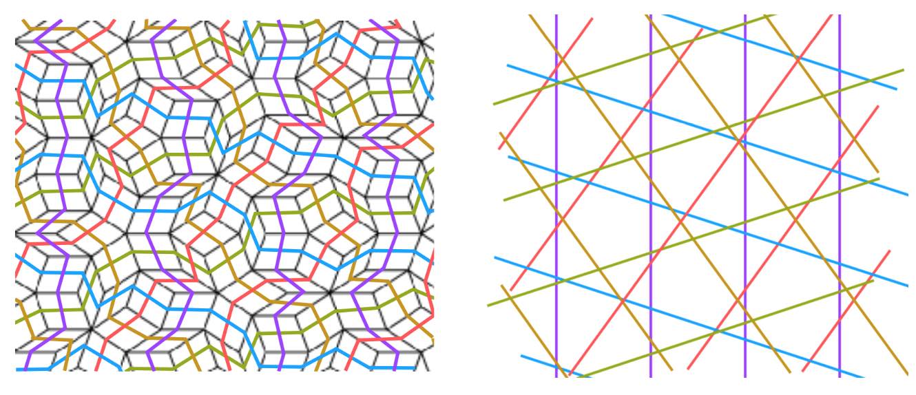
Last time we’ve seen that de Bruijn’s pentagrids determined the vertices of Penrose’s P3-aperiodic tilings.

These vertices can also be obtained by projecting a window of the standard hypercubic lattice $\mathbb{Z}^5$ by the cut-and-project-method.

We’ll bring in representation theory by forcing this projection to be compatible with a $D_5$-subgroup of the symmetries of $\mathbb{Z}^5$, which explains why Penrose tilings have a local $D_5$-symmetry.

The symmetry group of the standard $n$-dimensional hypercubic lattice
\[
\mathbb{Z} \vec{e}_1 + \dots + \mathbb{Z} \vec{e}_n \subset \mathbb{R}^n \]
is the hyperoctahedral group of all signed $n \times n$ permutation matrices
\[
B_n = C_2^n \rtimes S_n \]
in which all $n$-permutations $S_n$ act on the group $C_2^n = \{ 1,-1 \}^n$ of all signs. The signed permutation $n \times n$ matrix corresponding to an element $(\vec{a},\pi) \in B_n$ is given by
\[
T_{ij} = T(\vec{a},\pi)_{ij} = a_j \delta_{i,\pi(j)} \]
The represenation theory of $B_n$ was worked out in 1930 by the British mathematician and clergyman Alfred Young

We want to do explicit calculations in $B_n$ using a computational system such as GAP, so it is best to describe $B_n$ as a permutation subgroup of $S_{2n}$ via the morphism
\[
\tau((\vec{a},\pi))(k) = \begin{cases} \pi(k)+n \delta_{-1,a_k}~\text{if $1 \leq k \leq n$} \\
\pi(k-n)+n(1-\delta_{-1,a_{k-n}})~\text{if $n+1 \leq k \leq 2n$} \end{cases} \]
the image is generated by the permutations
\[
\begin{cases}
\alpha = (1,2)(n+1,n+2), \\
\beta=(1,2,\dots,n)(n+1,n+2,\dots,2n), \\
\gamma=(n,2n)
\end{cases}
\]
and to a permutation $\sigma \in \tau(B_n) \subset S_{2n}$ we assign the signed permutation $n \times n$ matrix $T_{\sigma}=T(\tau^{-1}(\pi))$.

We use GAP to set up $B_5$ from these generators and determine all its conjugacy classes of subgroups. It turns out that $B_5$ has no less than $953$ different conjugacy classes of subgroups.

gap> B5:=Group((1,2)(6,7),(1,2,3,4,5)(6,7,8,9,10),(5,10));
Group([ (1,2)(6,7), (1,2,3,4,5)(6,7,8,9,10), (5,10) ])
gap> Size(B5);
3840
gap> C:=ConjugacyClassesSubgroups(B5);;
gap> Length(C);
953

But we are only interested in the subgroups isomorphic to $D_5$. So, first we make a sublist of all conjugacy classes of subgroups of order $10$, and then we go through this list one-by-one and look for an explicit isomorphism between $D_5 = \langle x,y~|~x^5=e=y^2,~xyx=y \rangle$ and a representative of the class (or get a ‘fail’ is this subgroup is not isomorphic to $D_5$).

gap> C10:=Filtered(C,x->Size(Representative(x))=10);;
gap> Length(C10);
3
gap> s10:=List(C10,Representative);
[ Group([ (2,5)(3,4)(7,10)(8,9), (1,5,4,3,2)(6,10,9,8,7) ]),
Group([ (1,6)(2,5)(3,4)(7,10)(8,9), (1,10,9,3,2)(4,8,7,6,5) ]),
Group([ (1,6)(2,7)(3,8)(4,9)(5,10), (1,2,8,4,10)(3,9,5,6,7) ]) ]
gap> D:=DihedralGroup(10); gap> IsomorphismGroups(D,s10[1]);
[ f1, f2 ] -> [ (2,5)(3,4)(7,10)(8,9), (1,5,4,3,2)(6,10,9,8,7) ]
gap> IsomorphismGroups(D,s10[2]);
[ f1, f2 ] -> [ (1,6)(2,5)(3,4)(7,10)(8,9), (1,10,9,3,2)(4,8,7,6,5) ]
gap> IsomorphismGroups(D,s10[3]);
fail
gap> IsCyclic(s10[3]);
true

Of the three (conjugacy classes of) subgroups of order $10$, two are isomorphic to $D_5$, and the third one to $C_{10}$. Next, we have to transform the generating permutations into signed $5 \times 5$ permutation matrices using the bijection $\tau^{-1}$.
\[
\begin{array}{c|c}
\sigma & (\vec{a},\pi) \\
\hline
(2,5)(3,4)(7,10)(8,9) & ((1,1,1,1,1),(2,5)(3,4)) \\
(1,5,4,3,2)(6,10,9,8,7) & ((1,1,1,1,1)(1,5,4,3,2)) \\
(1,6)(2,5)(3,4)(7,10)(8,9) & ((-1,1,1,1,1),(2,5)(3,4)) \\
(1,10,9,3,2)(4,8,7,6,5) & ((-1,1,1,-1,1),(1,5,4,3,2))
\end{array}
\]
giving the signed permutation matrices
\[
\begin{array}{c|cc}
& x & y \\
\hline
A & \begin{bmatrix}
0 & 1 & 0 & 0 & 0 \\
0 & 0 & 1 & 0 & 0 \\
0 & 0 & 0 & 1 & 0 \\
0 & 0 & 0 & 0 & 1 \\
1 & 0 & 0 & 0 & 0 \end{bmatrix} &
\begin{bmatrix} 1 & 0 & 0 & 0 & 0 \\
0 & 0 & 0 & 0 & 1 \\
0 & 0 & 0 & 1 & 0 \\
0 & 0 & 1 & 0 & 0 \\
0 & 1 & 0 & 0 & 0 \end{bmatrix} \\
\hline
B & \begin{bmatrix}
0 & 1 & 0 & 0 & 0 \\
0 & 0 & 1 & 0 & 0 \\
0 & 0 & 0 & -1 & 0 \\
0 & 0 & 0 & 0 & 1 \\
-1 & 0 & 0 & 0 & 0 \end{bmatrix} &
\begin{bmatrix}
-1 & 0 & 0 & 0 & 0 \\
0 & 0 & 0 & 0 & 1 \\
0 & 0 & 0 & 1 & 0 \\
0 & 0 & 1 & 0 & 0 \\
0 & 1 & 0 & 0 & 0 \end{bmatrix}
\end{array}
\]
$D_5$ has $4$ conjugacy classes with representatives $e,y,x$ and $x^2$. the
character table of $D_5$ is
\[
\begin{array}{c|cccc}
& (1) & (2) & (2) & (5) \\
& 1_a & 5_1 & 5_2 & 2_a \\
D_5 & e & x & x^2 & y \\
\hline
T & 1 & 1 & 1 & 1 \\
V & 1 & 1 & 1 & -1 \\
W_1 & 2 & \tfrac{-1+ \sqrt{5}}{2} & \tfrac{-1 -\sqrt{5}}{2} & 0 \\
W_2 & 2 & \tfrac{-1 -\sqrt{5}}{2} & \tfrac{-1+\sqrt{5}}{2} & 0
\end{array}
\]
Using the signed permutation matrices it is easy to determine the characters of the $5$-dimensional representations $A$ and $B$
\[
\begin{array}{c|cccc}
D_5 & e & x & x^2 & y \\
\hline
A & 5 & 0 & 0 & 1 \\
B & 5 & 0 & 0 & -1
\end{array}
\]
decomosing into $D_5$-irreducibles as
\[
A \simeq T \oplus W_1 \oplus W_2 \quad \text{and} \quad B \simeq V \oplus W_1 \oplus W_2 \]
Representation $A$ realises $D_5$ as a rotation symmetry group of the hypercube lattice $\mathbb{Z}^5$ in $\mathbb{R}^5$, and next we have to find a $D_5$-projection $\mathbb{R}^5=A \rightarrow W_1 = \mathbb{R}^2$.

As a complex representation $A \downarrow_{C_5}$ decomposes as a direct sum of $1$-dimensional representations
\[
A \downarrow_{C_5} = V_1 \oplus V_{\zeta} \oplus V_{\zeta^2} \oplus V_{\zeta^3} \oplus V_{\zeta^4} \]
where $\zeta = e^{2 \pi i /5}$ and where the action of $x$ on $V_{\zeta^i}=\mathbb{C} v_i$ is given by $x.v_i = \zeta^i v_i$. The $x$-eigenvectors in $\mathbb{C}^5$ are
\[
\begin{cases}
v_0 = (1,1,1,1,1) \\
v_1 = (1,\zeta,\zeta^2,\zeta^3,\zeta^4) \\
v_2 =(1,\zeta^2,\zeta^4,\zeta,\zeta^3) \\
v_3 = (1,\zeta^3,\zeta,\zeta^4,\zeta^2) \\
v_4 = (1,\zeta^4,\zeta^3,\zeta^2,\zeta)
\end{cases}
\]
The action of $y$ on these vectors is given by $y.v_i = v_{5-i}$ because
\[
x.(y.v_i) = (xy).v_i=(yx^{-1}).v_i=y.(x^{-1}.v_i) = y.(\zeta^{-i} v_i) = \zeta^{-1} (y.v_i) \]
and therefore $y.v_i$ is an $x$-eigenvector with eigenvalue $\zeta^{5-i}$. As a complex $D_5$-representation, the factors of $A$ are therefore
\[
T = \mathbb{C} v_0, \quad W_1 = \mathbb{C} v_1 + \mathbb{C} v_4, \quad \text{and} \quad W_2 = \mathbb{C} v_2 + \mathbb{C} v_3 \]
But we want to consider $A$ as a real representation. As $\zeta^j = cos(\tfrac{2 \pi j}{5})+i~sin(\tfrac{2 \pi j}{5}) = c_j + i s_j$ hebben we can take the vectors in $\mathbb{R}^5$
\[
\begin{cases}
\frac{1}{2}(v_1+v_4) = (1,c_1,c_2,c_3,c_4)= u_1 \\
-\frac{1}{2}i(v_1-v_4) = (0,s_1,s_2,s_3,s_4) = u_2 \\
\frac{1}{2}(v_2+v_3) = (1,c_2,c_4,c1,c3)= w_1 \\
-\frac{1}{2}i(v_2-v_3) = (0,s_2,s_4,s_1,s_3)= w_2
\end{cases}
\]
and $A$ decomposes as a real $D_5$-representation with
\[
T = \mathbb{R} v_0, \quad W_1 = \mathbb{R} u_1 + \mathbb{R} u_2, \quad \text{and} \quad W_2 = \mathbb{R} w_1 + \mathbb{R} w_2 \]
and if we identify $\mathbb{C}$ with $\mathbb{R}^2$ via $z \leftrightarrow (Re(z),Im(z))$ we can describe the $D_5$-projection morphism $\pi_{W_1}~:~\mathbb{R}^5=A \rightarrow W_1=\mathbb{R}^2$ via
\[ (y_0,y_1,y_2,y_3,y_4) \mapsto y_0+y_1 \zeta + y_2 \zeta^2 + y_3 \zeta^3 + y_4 \zeta^4 = \sum_{i=0}^4 y_i (c_i,s_i) \]
Note also that $W_1$ is the orthogonal complement of $T \oplus W_2$, so is equal to the linear subspace in $\mathbb{R}^5$ determined by the three linear equations
\[
\begin{cases}
\sum_{i=0}^4 x_i = 0 \\
\sum_{i=0}^4 c_{2i} x_i = 0 \\
\sum_{i=0}^4 s_{2i} x_i = 0
\end{cases}
\]

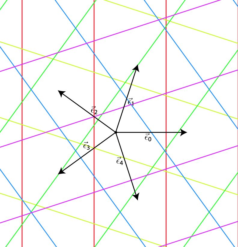
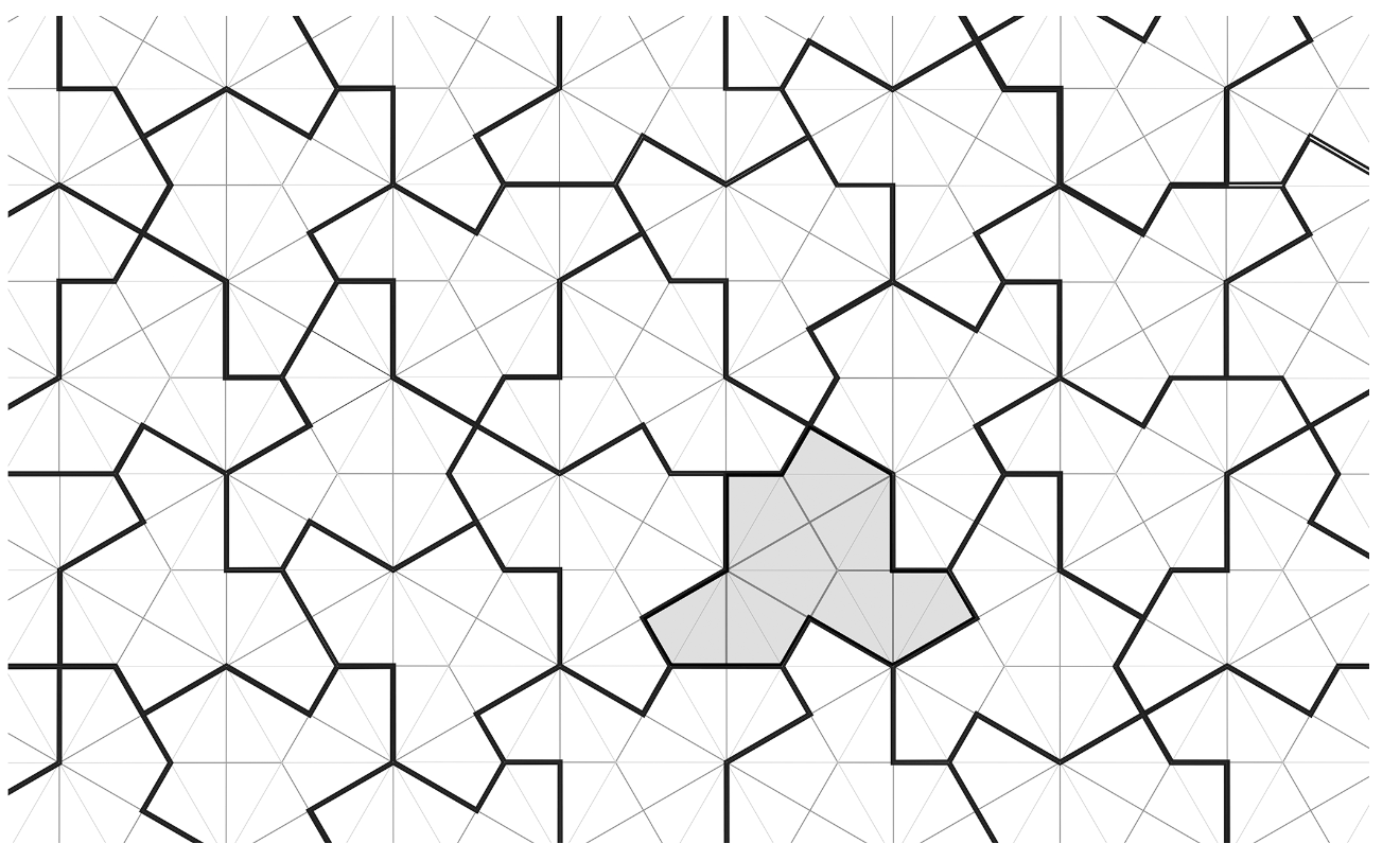
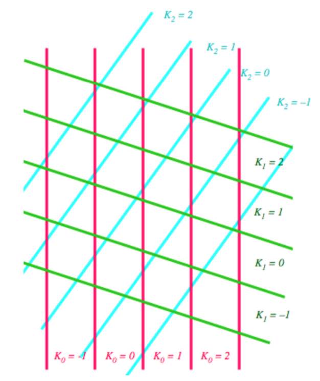
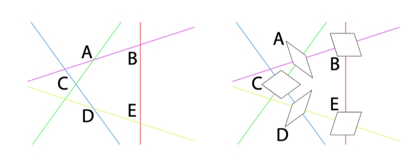
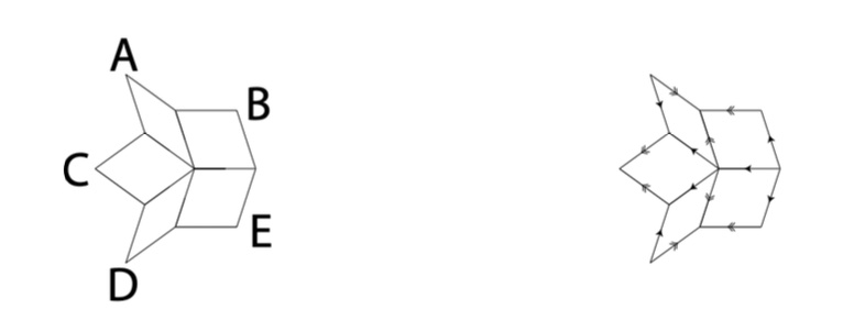
Okay, now take the Rhombic tiling corresponding to the regular pentagrid defined by $\gamma_0, \dots, \gamma_4$ satisfying $\sum_{i=0}^4 \gamma_i = 0$. Let $\vec{k}=(k_0,\dots,k_4) \in \mathbb{Z}^5$ and define the open hypercube $H_{\vec{k}}$ corresponding to $\vec{k}$ as the set of points
\[
(x_0,\dots,x_4) \in \mathbb{R}^5~:~\forall 0 \leq i \leq 4~:~k_i – 1 < x_i < k_i \] From the vector $\vec{\gamma} = (\gamma_0,\dots,\gamma_4)$ determining the Rhombic tiling we define the $2$-dimensional plane $P_{\vec{\gamma}}$ in $\mathbb{R}^5$ given by the equations \[ \begin{cases} \sum_{i=0}^4 x_i = 0 \\ \sum_{i=0}^4 c_{2i} (x_i - \gamma_i) = 0 \\ \sum_{i=0}^4 s_{2i} (x_i - \gamma_i) = 0 \end{cases} \] The point being that $P_{\vec{\gamma}}$ is the linear plane $W_1$ in $\mathbb{R}^5$ translated over the vector $\vec{\gamma}$, so it is parallel to $W_1$. Here's the punchline:

de Bruijn’s theorem: The vertices of the Rhombic tiling produced by the regular pentagrid with parameters $\vec{\gamma}=(\gamma_0,\dots,\gamma_4)$ are the points
\[
\sum_{i=0}^4 k_i (c_i,s_i) \]
with $\vec{k}=(k_0,\dots,k_4) \in \mathbb{Z}^5$ such that $H_{\vec{k}} \cap P_{\vec{\gamma}} \not= \emptyset$.

To see this, let $\vec{x} = (x_0,\dots,x_4) \in P_{\vec{\gamma}}$, then $\vec{x}-\vec{\gamma} \in W_1$, but then there is a vector $\vec{y} \in \mathbb{R}^2$ such that
\[
x_j – \gamma_j = \vec{y}.\vec{v}_j \quad \forall~0 \leq j \leq 4 \]
But then, with $k_j=\lceil \vec{y}.\vec{v}_j + \gamma_j \rceil$ we have that $\vec{x} \in H_{\vec{k}}$ and we note that $V(\vec{y}) = \sum_{i=0}^4 k_i \vec{v}_i$ is a vetex of the Rhombic tiling associated to the regular pentagrid parameters $\vec{\gamma}=(\gamma_0,\dots,\gamma_4)$.

Here we used regularity of the pentagrid in order to have that $k_j=\vec{y}.\vec{v}_j + \gamma_j$ can happen for at most two $j$’s, so we can manage to vary $\vec{y}$ a little in order to have $\vec{x}$ in the open hypercube.

Here’s what we did so far: we have identified $D_5$ as a group of rotations in $\mathbb{R}^5$, preserving the hypercube-lattice $\mathbb{Z}^5$ in $\mathbb{R}^5$. If the $2$-plane $P_{\vec{\gamma}}$ is left stable under these rotations, then because rotations preserve distances, also the subset of lattice-points
\[
S_{\vec{\gamma}} = \{ (k_0,\dots,k_4)~|~H_{\vec{k}} \cap P_{\vec{\gamma}} \not= \emptyset \} \subset \mathbb{Z}^5 \]
is left stable under the $D_5$-action. But, because the map
\[
(k_0,\dots,k_4) \mapsto \sum_{i=0}^4 k_i (c_i,s_i) \]
is the $D_5$-projection map $\pi : A \rightarrow W_1$, the vertices of the associated Rhombic tiling must be stable under the $D_5$-action on $W_1$, meaning that the Rhombic tiling should have a global $D_5$-symmetry.

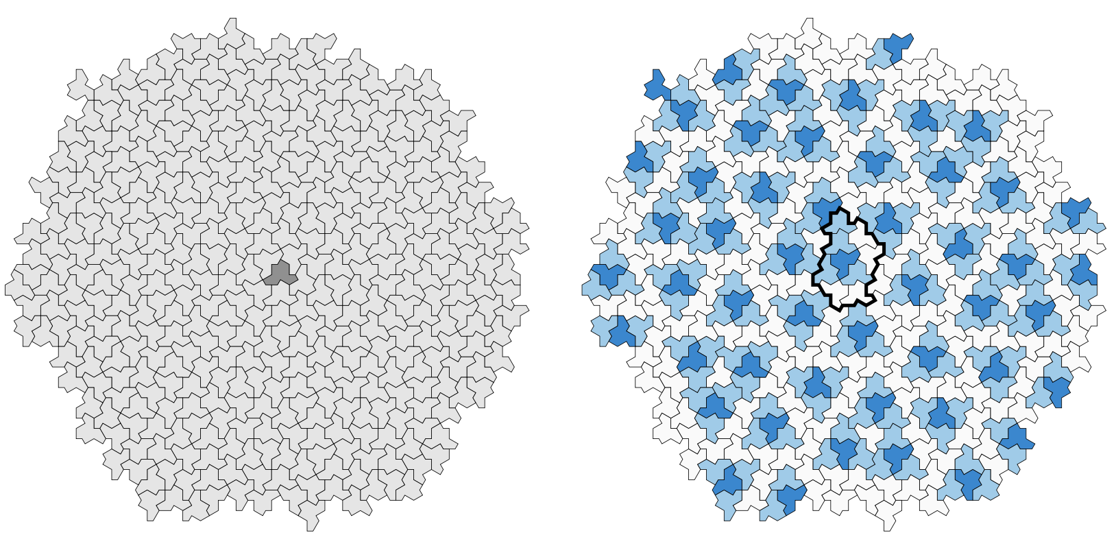
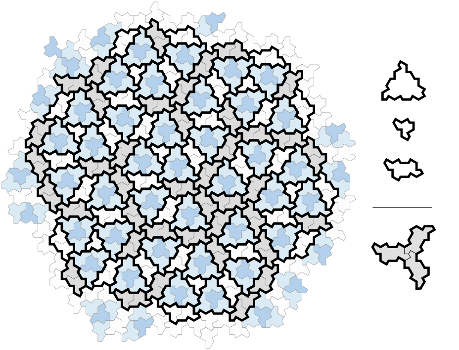
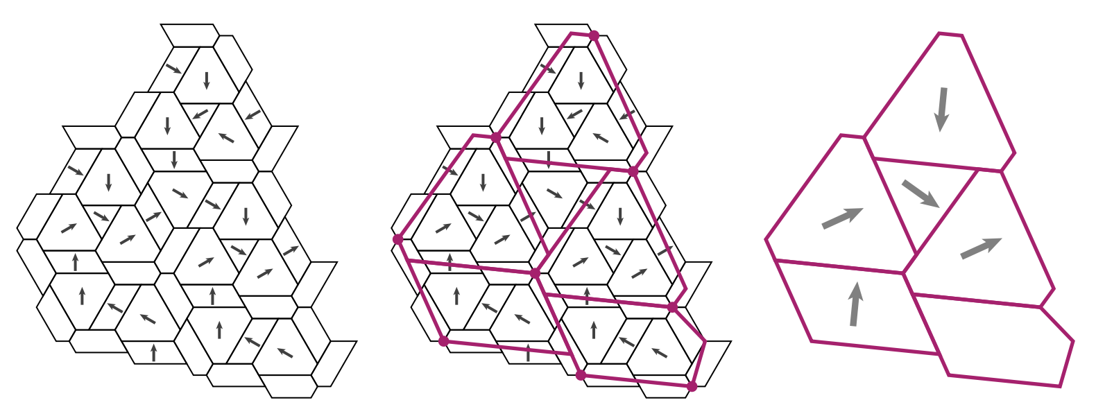
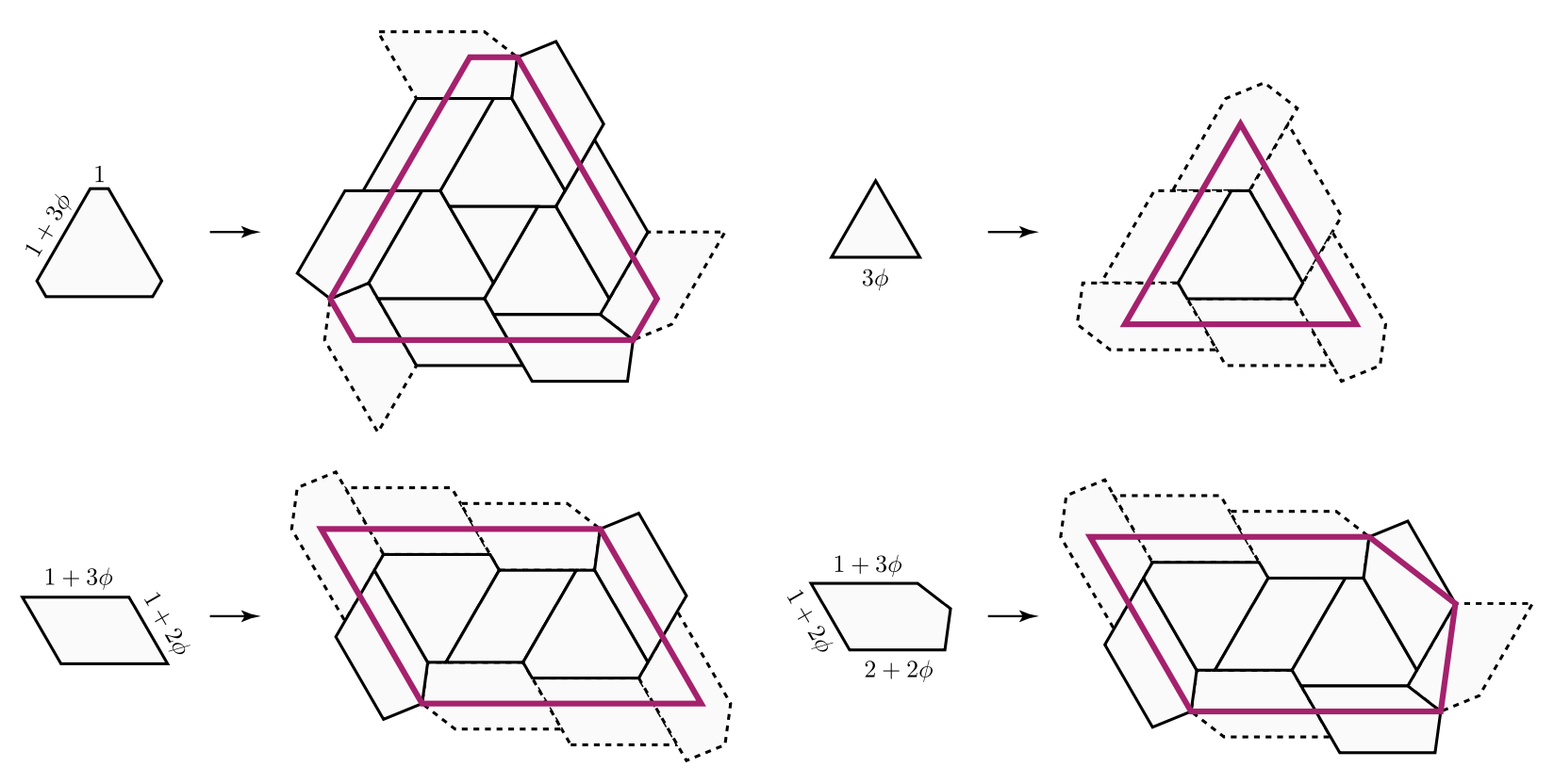
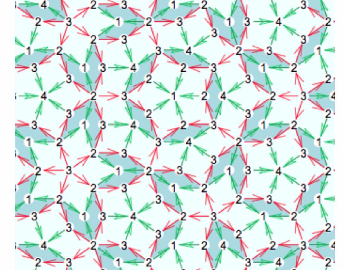
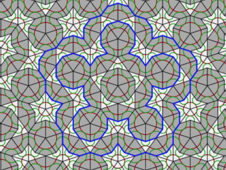
Sadly, the only plane $P_{\vec{\gamma}}$ left stable under all rotations of $D_5$ is when $\vec{\gamma} = \vec{0}$, which is an exceptionally singular pentagrid. If we project this situation we do indeed get an image with global $D_5$-symmetry

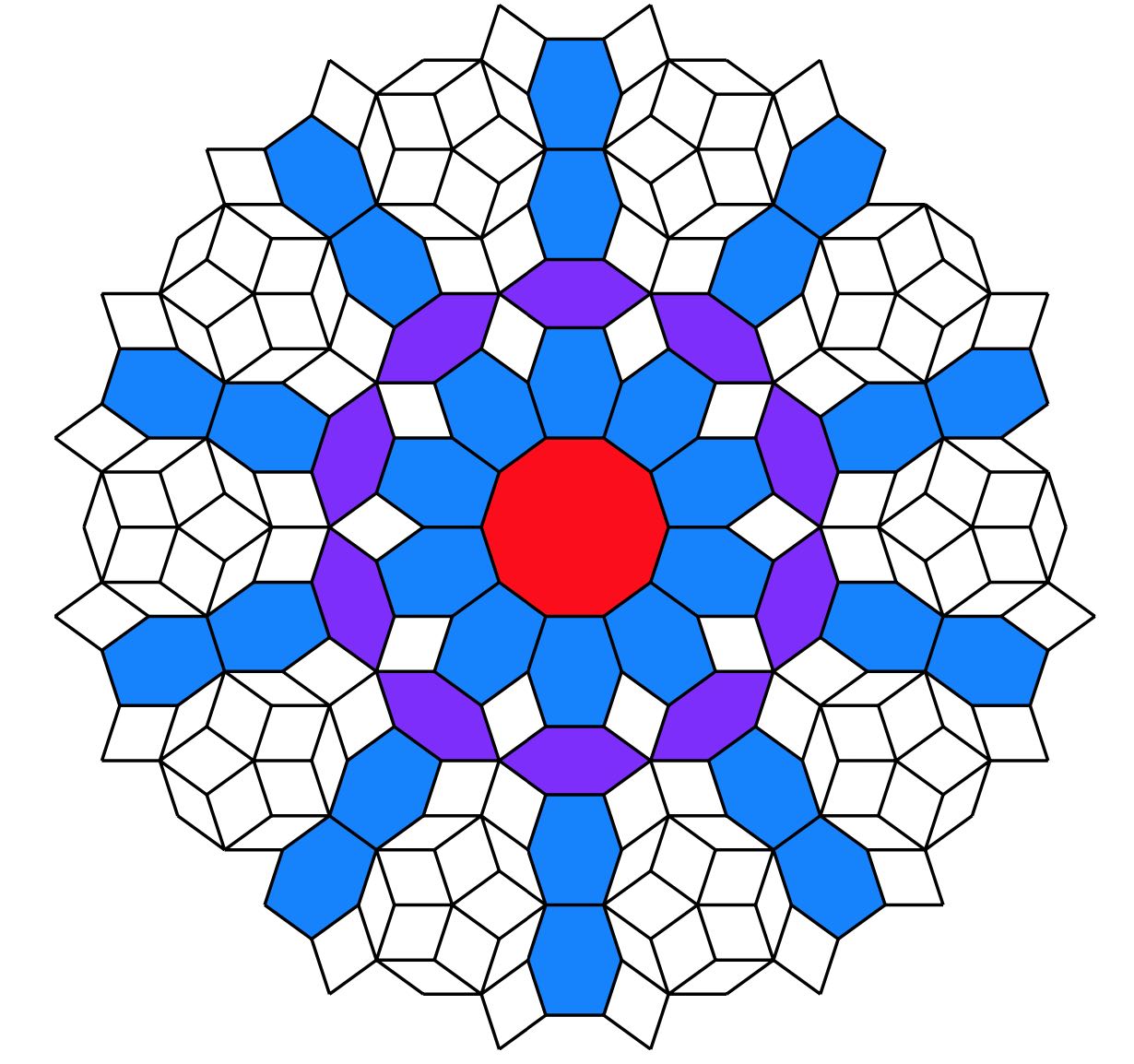
but it is not a Rhombic tiling. What’s going on?

Because this post is already dragging on for far too long (TL;DR), we’ll save the investigation of projections of singular pentagrids, how they differ from the regular situation, and how they determine multiple Rhombic tilings, for another time.

Leave a Comment

de Bruijn’s pentagrids

Published March 11, 2021 by lievenlb

In a Rhombic tiling (aka a Penrose P3 tiling) we can identify five ribbons.

Opposite sides of a rhomb are parallel. We may form a ribbon by attaching rhombs along opposite sides. There are five directions taken by sides, so there are five families of ribbons that do not intersect, determined by the side directions.

Every ribbon determines a skeleton curve through the midpoints of opposite sides of the rhombs. If we straighten these skeleton curves we get a de Bruijn’s pentagrid.

A pentagrid is a grid of the plane consisting of five families of parallel lines, at angles multiples of $72^o = 360^o/5$, and with each family consisting of parallel lines with a spacing given by a number $\gamma_i$ for $0 \leq i \leq 4$, satisfying
\[
\gamma_0+\gamma_1+\gamma_2+\gamma_3+\gamma_4=0 \]

The points of the plane in the $j$-th family of the pentagrid are
\[
\{ \vec{x} \in \mathbb{R}^2~|~\vec{x}.\vec{v}_j + \gamma_j \in \mathbb{Z} \} \]
where $\vec{v}_j = \zeta^j = (cos(2 \pi j/5),sin(2 \pi j/5))$.

A pentagrid is regular if no point in $\mathbb{R}^2$ belongs to more than two of the five grids. For almost all choices $\gamma_0,\dots,\gamma_4$ the corresponding pentagrid is regular. The pentagrid coordinates of a point $\vec{x} \in \mathbb{R}^2$ are the five integers $(K_0(\vec{x}),\dots,K_4(\vec{x}) \in \mathbb{Z}^5$ defined by
\[
K_j(\vec{x}) = \lceil \vec{x}.\vec{v}_j + \gamma_j \rceil \]
with $\lceil r \rceil$ the smallest integer greater of equal to $r$, and clearly the function $K_j(\vec{x})$ is constant in regions between the $j$-th grid lines.

With these pentagrid-coordinates one can associate a vertex to any point $\vec{x} \in \mathbb{R}^2$
\[
V(\vec{x}) = \sum_{j=0}^4 K_j(\vec{x}) \vec{v}_j \]
which is constant in regions between grid lines.

Here’s de Bruijn‘s result:

For $\vec{x}$ running over $\mathbb{R}^2$, the vertices $V(\vec{x})$ coming from a pentagrid determine a Rhombic tiling of the plane. Even better, every Rhombic tiling comes from a pentagrid.

We’ll prove this for regular pentagrids (the singular case follows from a small deformation).

Any intersection point $\vec{x}_0$ of the pentagrid belongs to exactly two families of parallel lines, so we have two integers $r$ and $s$ with $0 \leq r < s \leq 4$ and integers $k_r,k_s \in \mathbb{Z}$ such that $\vec{x}_0$ is determined by the equations \[ \begin{cases} \vec{x}.\vec{v}_r + \gamma_r = k_r \\ \vec{x}.\vec{v}_s + \gamma_s = k_s \end{cases} \] In a small neighborhood of $\vec{x}_0$, $V(\vec{x})$ takes the values of four vertices of a rhomb. These vertices are associated to the $5$-tuples in $\mathbb{Z}^5$ given by \[ (K_0(\vec{x}_0),\dots,K_4(\vec{x}_0))+\epsilon_1 (\delta_{0r},\dots,\delta_{4r})+\epsilon_2 (\delta_{0s},\dots,\delta_{4s}) \] with $\epsilon_1,\epsilon_2 \in \{ 0,1 \}$. So, the intersection points of the regular pentagrid lines correspond to rhombs, and the regions between the grid lines (which are called meshes) correspond to vertices, whose positions are given by $V(\vec{x})$.

Observe that these four vertices give a thin rhombus if the angle between $\vec{v}_r$ and $\vec{v}_s$ is $144^o$ and determine a thick rhombus if the angle is $72^o$.

Not all pentagrid coordinates $(k_0,\dots,k_4)$ occur in the tiling though. For $\vec{x} \in \mathbb{R}^2$ we have
\[
K_j(\vec{x}) = \vec{x}.\vec{v}_j + \gamma_j + \lambda_j(\vec{x}) \]
with $0 \leq \lambda_j(\vec{x}) < 1$. In a regular pentagrid at most two of the $\lambda_j(\vec{x})$ can be zero and so we have \[ 0 < \lambda_0(\vec{x}) + \dots + \lambda_4(\vec{x}) < 5 \] and we have assumed that $\gamma_0 + \dots + \gamma_4 = 0$, giving us \[ \sum_{j=0}^4 K_j(\vec{x}) = \vec{x}.(\sum_{j=0}^4 \vec{v}_j) + \sum_{j=0}^4 \gamma_j + \sum_{j=0}^4 \lambda_j(\vec{x}) = \sum_{j=0}^4 \lambda_j(\vec{x}) \] The left hand side must be an integers and the right hand side a number strictly between $0$ and $5$. This defines the index of a vertex
\[
ind(\vec{x}) = \sum_{j=0}^4 K_j(\vec{x}) \in \{ 1,2,3,4 \} \]
Therefore, every vertex in the tiling may be represented as
\[
k_0 \vec{v}_0 + \dots + k_4 \vec{v}_4 \]
with $(k_0,\dots,k_4) \in \mathbb{Z}^5$ satisfying $\sum_{j=0}^4 k_j \in \{ 1,2,3,4 \}$. If we move a point along the edges of a rhombus, we note that the index increases by $1$ in the directions of $\vec{v}_0,\dots,\vec{v}_4$ and decreases by $1$ in the directions $-\vec{v}_0,\dots,-\vec{v}_4$.

It follows that the index-values of the vertices of a thick rhombus are either $1$ and $3$ at the $72^o$ angles and $2$ at the $108^o$ angles, or they are $2$ and $4$ at the $72^o$ angles, and $3$ at the $108^o$ angles. For a thin rhombus the index-values must be either $1$ and $3$ at the $144^o$ angles and $2$ at the $36^o$ angles, or $2$ and $4$ at the $144^o$ angles and $3$ at the $36^o$ angles.

We still have to show that this gives a legal Rhombic tiling, that is, that the gluing restrictions of Penrose’s rhombs are satisfied.

We do this by orienting and colouring the edges of the thin and thick rhombus towards the vertex defined by the semi-circles on the rhombus-pieces. Edges connecting a point of index $3$ to a point of index $2$ are coloured red, edges connecting a point of index $1$ to a point of index $2$, or connecting a point of index $3$ to one of index $4$ are coloured blue.

We orient green edges pointing from index $2$ to index $1$, or from index $3$ to index $4$. As this orientation depends only on the index-values of the vertices, two rhombs sharing a common green edge also have the same orientation on that edge.

On each individual rhomb, knowing the green edges and their orientation forced the red edges and their orientation, but we still have to show that if two rhombs share a common red edge, this edge has the same orientation on both (note in the picture above that a red edge can both flow from $2$ to $3$ as well as from $3$ to $2$).

From the gluing conditions of Penrose’s rhombs we see that if $PQ$ be a red edge, in common to two rhombs, and these rhombs have angle $\alpha$ resp. $\beta$ in $P$, then $\alpha$ and $\beta$ must be both less that $90^o$ or both bigger than $90^o$. We translate this in terms of the pentragrid.

The two rhombs correspond to two intersection points $A$ and $B$, and we may assume that they both lie on a line $l$ of family $0$ of parallel lines (other cases are treated similarly by cyclic permutation), and that $A$ is an intersection with a family $p$-line and $B$ with a family $q$-line, with $p,q \in \{ 1,2,3,4 \}$. The interval $AB$ crosses the unique edge common to the two rhombs determined by $A$ and $B$, and we call the interval $AB$ red if $\sum_j K_j(\vec{x})$ is $2$ on one side of $AB$ and $3$ on the other side. The claim about the angles $\alpha$ and $\beta$ above now translates to: if $AB$ is red, then $p+q$ is odd (in the picture above $p=1$ and $q=2$).

By a transformation we may assume that $\gamma_0=0$ and that $l$ is the $Y$-axis. For every $y \in \mathbb{R}$ we then get
\[
\begin{cases}
K_1(0,y) = \lceil y .sin(2 \pi/5) + \gamma_1 \rceil \\
K_2(0,y) = \lceil y .sin(4 \pi/5) + \gamma_2 \rceil \\
K_3(0,y) = \lceil -y .sin(4 \pi/5) + \gamma_3 \rceil \\
K_4(0,y) = \lceil -y .sin(2 \pi/5) + \gamma_4 \rceil
\end{cases}
\]
and $\gamma_1+\gamma_4$ and $\gamma_2+\gamma_3$ are not integers (otherwise the pentagrid is not regular). If $y$ runs from $-\infty$ to $+\infty$ we find that
\[
K_1(0,y)+K_4(0,y) – \lceil \gamma_1 + \gamma_4 \rceil = \begin{cases} 0 \\ 1 \end{cases} \]
with jumps from $0$ to $1$ at places where $(\lceil \gamma_1 + \gamma_4 \rceil – \gamma_1)/sin(2 \pi/5) \in \mathbb{Z}$ and from $1$ to $0$ when $\gamma_4/sin(2 \pi/5) \in \mathbb{Z}$. (A similar result holds replacing $K_1,K_4,\gamma_1,\gamma_4,sin(2 \pi/5)$ by $K_2,K_3,\gamma_2,\gamma_3,sin(4 \pi/5)$.

Because the points on $l$ intersecting with $1$-family and $4$-family gridlines alternate (and similarly for $2$- and $3$-family gridlines) we know already that $p \not= q$. If we assume that $p+q$ is even, we have two possibilities, either $\{p,g \}=\{ 1,3 \}$ or $\{ 2,4 \}$. As $\gamma_0=0$ we have $\gamma_1+\gamma_2+\gamma_3+\gamma_4=0$ and therefore
\[
\lceil \gamma_1 + \gamma_4 \rceil + \lceil \gamma_2+\gamma_3 \rceil = 1 \]
It then follows that $K_1(0,y)+K_2(0,y)+K_3(0,y)+K_4(0,y) = 1$ or $3$ between the points $A$ and $B$. Therefore $K_0(y,0) + \dots + K_4(0,y)$ is either $1$ on the left side and $2$ on the right side, or is $3$ on the left side and $4$ on the right side, so $AB$ must be green, a contradiction. Therefore, $p+q$ is odd, and the orientation of the red edge in both rhombs is the same. Done!

An alternative way to see this correspondence between regular pentagrids and Rhombic tilings as as follows. To every intersection of two gridlines we assign a rhombus, a thin one if they meet at an acute angle of $36^o$ and a thich one if this angle is $72^o$, with the long diagonal dissecting the obtuse angle.

Do this for all intersections, surrounding a given mesh.

Attach the rhombs by translating them towards the mesh, and finally draw the colours of the edges.

Another time, we will connect this to the cut-and-project method, using the representation theory of $D_5$.

Leave a Comment

GoV 2 : Viruses and quasi-crystals

Published February 26, 2021 by lievenlb

If you look around for mathematical theories of the structure of viruses, you quickly end up with the work of Raidun Twarock and her group at the University of York.

We’ve seen her proposal to extend the Caspar-Klug classification of viruses. Her novel idea to distribute proteins on the viral capsid along Penrose-like tilings shouldn’t be taken too literally. The inherent aperiodic nature of Penrose tiles doesn’t go together well with perfect tilings of the sphere.

Instead, the observation that these capsid tilings resemble somewhat Penrose tilings is a side-effect of another great idea of the York group. Recently, they borrowed techniques from the theory of quasicrystals to gain insight in the inner structure of viruses, in particular on the interaction of the capsid with the genome.

By the crystallographic restriction theorem no $3$-dimensional lattice can have icosahedral symmetry. But, we can construct aperiodic structures (quasicrystals) which have local icosahedral structure, much like Penrose tilings have local $D_5$-symmetry

This is best explained by de Bruijn‘s theory of pentagrids (more on that another time). Here I’ll just mention the representation-theoretic idea.

The isometry group of the standard $5$-dimensional lattice $\mathbb{Z}^5$ is the group of all signed permutation $5 \times 5$ matrices $B_5$ (Young’s hyperoctahedral group). There are two distinct conjugacy classes of subgroups in $B_5$ isomorphic to $D_5$, one such subgroup generated by the permutation matrices
\[
x= \begin{bmatrix}
0 & 1 & 0 & 0 & 0 \\
0 & 0 & 1 & 0 & 0 \\
0 & 0 & 0 & 1 & 0 \\
0 & 0 & 0 & 0 & 1 \\
1 & 0 & 0 & 0 & 0 \end{bmatrix} \qquad \text{and} \qquad
y = \begin{bmatrix} 1 & 0 & 0 & 0 & 0 \\
0 & 0 & 0 & 0 & 1 \\
0 & 0 & 0 & 1 & 0 \\
0 & 0 & 1 & 0 & 0 \\
0 & 1 & 0 & 0 & 0 \end{bmatrix} \]
The traces of $x,x^2$ and $y$, together with the character table of $D_5$ tell us that this $5$-dimensional $D_5$-representation splits as the direct sum of the trivial representation and of the two irreducible $2$-dimensional representations.
\[
\mathbb{R}^5 = A \simeq T \oplus W_1 \oplus W_2 \]
with $T = \mathbb{R} d$, $W_1 = \mathbb{R} u_1 + \mathbb{R} u_2$ and $W_2 = \mathbb{R} w_1 + \mathbb{R} w_2$ where
\[
\begin{cases}
(1,1,1,1,1)=d \\
(1,c_1,c_2,c_3,c_4)= u_1 \\
(0,s_1,s_2,s_3,s_4) = u_2 \\
(1,c_2,c_4,c1,c3)= w_1 \\
(0,s_2,s_4,s_1,s_3)= w_2
\end{cases}
\]
and $c_j=cos(2\pi j/5)$ and $s_j=sin(2 \pi/5)$. We have a $D_5$-projection
\[
\pi : A \rightarrow W_1 \quad (y_0,\dots,y_4) \mapsto \sum_{i=0}^4 y_i(c_i u_1+s_i u_2) \]
The projection maps the vertices of the $5$-dimensional hypercube to a planar configuration with $D_5$-symmetry.

de Bruijn’s results say that if we take suitable ‘windows’ of lattice-points in $\mathbb{Z}^5$ and project them via the $D_5$-equivariant map $\pi$ onto the plane, then the images of these lattice points become the vertices of a rhombic Penrose tiling (and we get all such tilings by choosing our window carefully).

This explains why Penrose tilings have a local $D_5$-symmetry. I’ll try to come back to de Bruijn’s papers in future posts.

But, let’s go back to viruses and the work of Twarock’s group using methods from quasicrystals. Such aperiodic structures with a local icosahedral symmetry can be constructed along similar lines. This time one starts with the standard $6$-dimensional lattice $\mathbb{Z^6}$ with isometry group $B_6$ (signed $6 \times 6$ permutation matrices).

This group has three conjugacy classes of subgroups isomorphic to $A_5$, but for only one of them this $6$-dimensional representation decomposes as the direct sum of the two irreducible $3$-dimensional representations of $A_5$ (the decompositions in the two other cases contain an irreducible of dimension $4$ or $5$ together with trivial factor(s)). A representant of the crystallographic relevant case is given by the signed permutation matrices
\[
x= \begin{bmatrix}
0 & 1 & 0 & 0 & 0 & 0 \\
1 & 0 & 0 & 0 & 0 & 0 \\
0 & 0 & 0 & -1 & 0 & 0 \\
0 & 0 & -1 & 0 & 0 & 0 \\
0 & 0 & 0 & 0 & -1 & 0 \\
0 & 0 & 0 & 0 & 0 & -1
\end{bmatrix} \qquad \text{and} \qquad y=
\begin{bmatrix}
0 & 0 & 1 & 0 & 0 & 0 \\
1 & 0 & 0 & 0 & 0 & 0 \\
0 & 1 & 0 & 0 & 0 & 0 \\
0 & 0 & 0 & 0 & -1 & 0 \\
0 & 0 & 0 & 0 & 0 & 1 \\
0 & 0 & 0 & -1 & 0 & 0
\end{bmatrix} \]

Again, using suitable windows of $\mathbb{Z}^6$-lattice points and using the $A_5$-equivariant projection to one of the two $3$-dimensional components, one obtains quasicrystals with local $A_5$-symmetry.

In this $3$-dimensional case the replacements of the thick and thin rhombi are these four parallellepipeda, known as the Amman blocks

which must be stacked together obeying the gluing condition that dots of the same colour must be adjacent.

Has anyone looked at a possible connection between the four Amman blocks (which come in pairs) and the four (paired) nucleotides in DNA? Just an idle thought…

These blocks grow into quasicrystals with local icosahedral symmetry.

The faces on the boundary of such a sphere-like quasicrystal then look a lot like a Penrose tiling.

How can we connect these group and representation-theoretic ideas to the structure of viruses? Here’s another thought-provoking proposal coming from the York group.

Take the $A_5$ subgroup of the hyperoctahedral group in six dimensiona $B_6$ generated by the above two matrices (giving a good $A_5$-equivariant projection $\pi$ to three dimensional space) and consider an intermediate group
\[
A_5 \subsetneq G \subseteq B_6 \]
Take a point in $\mathbb{R}^6$ and look at its orbit under the isometries of $G$, then all these points have the same distance from the origin in $\mathbb{R}^6$. Now, project this orbit under $\pi$ to get a collection of points in $\mathbb{R}^3$.

As $\pi$ is only $A_5$-equivariant (and not $G$-equivariant) the image points may lie in different shells from the origin. We can try to relate these shells of points to observational data on the inner structures of viruses.

Here’s a pretty convincing instance of such a correlation, taken from the thesis by Emilio Zappa “New group theoretical methods for applications in virology and quasicrystals”.

This is the inner structure of the Hepatitis B virus, showing the envelope (purple), capsid protein (cream) and genome (light blue). The coloured dots are the image points in the different shells around the origin.

Do viruses invade us from the sixth dimension??

Leave a Comment