Skip to content →

neverendingbooks Posts

bandwidth measures


One day (hopefully) lots of MP3, JPEG and perhaps even
MPEG-files will be flying around our wireless home-network. But I
didn’t have any idea of how much data I could cram through the
Airport-connections. To estimate the available bandwith of a
network there is a nice free tool around, iperf of which you can download binaries for
almost any platform including OS X. So click on the MacOS X (Darwin 6.4)
binary button half way on the iperf-page and you get a Desktop
iperf-1.7.0-powerpc-apple-darwin6.4 Folder
which you may rename to
just iperf. Do this on two computers connected to the
Airport-network you want to measure. Now, decide which of the two will
play the ‘server’ and which the ‘client’ (the end result does not
depend on this choice). So fire up the Terminal of the serving
computer and type

sudo ~/Desktop/iperf/iperf -s

and you will
get a message saying that the server is listening on TCP port 5001. Go
to the SystemPreferences/Network to obtain the IP-address of the server
(say it is 10.0.1.5) . Walk over to the ‘client’-computer and type
into its Terminal

sudo ~/Desktop/iperf/iperf -c 10.0.1.5
-r

and after a few moments it will compute the bandwidth of the
connection for you. Here is a sample output of two Airport-card
iMacs connected to the same Airport-Extreme base station :

iMacLieven:~/Desktop/iperf lieven$ ./iperf
-s ------------------------------------------------------------\r\
nServer listening on TCP port 5001 TCP window size: 64.0 KByte
(default) -----------------------------------------------------------
- [  4] local 10.0.1.2 port 5001 connected with 10.0.1.7 port
49245 [ ID] Interval       Transfer     Bandwidth [  4]  0.0-10.3
sec  2.77 MBytes  2.27
Mbits/sec -----------------------------------------------------------
- Client connecting to 10.0.1.7, TCP port 5001 TCP window size:
65.0 KByte
(default) -----------------------------------------------------------
- [  4] local 10.0.1.2 port 49515 connected with 10.0.1.7 port
5001 [ ID] Interval       Transfer     Bandwidth [  4]  0.0-10.2
sec  2.73 MBytes  2.23 Mbits/sec indicating a bandwidth of approximately
2.25Mbits/sec. If we replay the same game with two
AirportExtreme-card iMacs on the same network we can nearly
triple (!) the bandwidth : 
[eMacAnn:~] lieven% cd
Desktop/iperf [eMacAnn:~/Desktop/iperf] lieven% ./iperf
-s ------------------------------------------------------------\r\
nServer listening on TCP port 5001 TCP window size: 64.0 KByte
(default) -----------------------------------------------------------
- [  4] local 10.0.1.5 port 5001 connected with 10.0.1.6 port
49314 [ ID] Interval       Transfer     Bandwidth [  4]  0.0-10.0
sec  8.50 MBytes  7.11
Mbits/sec -----------------------------------------------------------
- Client connecting to 10.0.1.6, TCP port 5001 TCP window size:
65.0 KByte
(default) -----------------------------------------------------------
- [  4] local 10.0.1.5 port 49320 connected with 10.0.1.6 port
5001 [ ID] Interval       Transfer     Bandwidth [  4]  0.0-10.9
sec  7.07 MBytes  5.45 Mbits/sec

However, if these two
AirportExtrame-card computers connect to each other via the
Graphite-Airport base station the bandwidth drops to a meagre 1.9
Mbits/sec which is roughly the same as two Airport-card computers
connecting (which gave me 2.45 Mbits/s). Anyway, there is no immediate
problem with bandwidth on either network for what I have in mind.
Another important number to know is the real speed of our
internet-connection (for instance if I want to replace our old router by
a better documented one and have a measure for the in/decrease of the
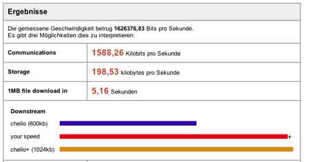
connection-speed). Here, a good URL is performance.chello.at which offers two tests :
String and String SSI. The later one has a graphical
resulting page such as

Leave a Comment

google spammers


In the GoogleMatrix I tried to understand the concept
of the PageRank algorithm that Google uses to list pages according to
their \’importance\’. So, if you want your webpage to come out first in
a certain search, you have to increase your PageRank-value (which
normally is a measure of webpages linking to your page) artificially. A
method to achieve this is by link spamming, that is if page A is
to webpage of which you want to increase the PageRank value, take a page
B (either under your control or that of a friend webmaster) and add a
dummy link page B -> page A. To find out the effect of this on the
PageRank and how the second eigenvalue of the GoogleMatrix is able to
detect such constructs let us set up a micro-web consisting of
just 3 pages with links 1->2 and 1->3. The corresponding GoogleMatrix
(with c=0.85 and v=(1/3,1/3,1/3) is

1/3   1/20   1/20 1/3   9/10 
 1/20 1/3   1/20   9/10

which has eigenvalues 1,0.85 and 0.28.
The eigenvector with eigenvalue 1 (the PageRank) is equal to (0.15,1,1)
so page 2 and page 3 are equally important to Google and if we scale
PageRank such that it adds up to 100% over all pages, the relative
importance values are 6,9%,46,5% and 46,5%. In this case the eigenvector
corresponding to the second eigenvalue 0.85 is (0,-1,1) and hence
detects the two leaf-nodes. Now, assume the owner of page 2 sets up a
link spam by creating page 4 and linking 4->3, then the corresponding
GoogleMatrix (with v=(1/4,1/4,1/4,1/4)) is

77/240   3/80   3/80  
3/80 77/240   71/80   3/80   37/80 77/240   3/80   71/80  
3/80  3/80   3/80   3/80   37/80

which has eigenvalues
1,0.85,0.425 and 0.283. The PageRank eigenvector with eigenvalue 1 is
in this case is (0.8,8.18,5.35,1) or in relative importance % we have
(4.9%,50.1%,32.7%,6.1%) and we see that the spammer achieved his/her
goal. The eigenvector corresponding to the second eigenvalue is
(0,-1,1,0) which again gives the leaf-nodes and the eigenvector of the
third eigenvalue is (0,-1,0,1) and detects the spam-construct.

Leave a Comment

an even better LaTeX system

A
previous post the best LaTeX system was a commercial for Gerben
Wierda’s i-Installer to get a working tetex
distribution. I’ve been working happily with this TeX-system for two
years now but recently run into a few (minor) problems. In the process
of solving these problems I created myself a second tetex-system
more or less by accident. This is what happened. On the computer at the
university I once got fun packages running such as a chess-, go-
and Feynman diagrams-package but somehow I cannot reproduce this
on my home-machine, I get lots of errors with missing fonts etc. As I
really wanted to TeX some chess-diagrams I went surfing for the most
recent version of the chess-package and found one for Linux and
one under the Fink-project : the chess-tex package. So, I did a

sudo fink
install chess-tex

forgetting that in good Fink-tradition you can
only install a package by installing at the same time all packages
needed to run it, so I was given a whole list of packages that Fink
wanted to install including a full tetex-system. Did I want to
continue? Well, I had to think on that for a moment but realized that
the iTex-tree was living under /usr/local whereas Fink
creates trees under /sw so there should not really be a problem,
so yes let’s see what happens. It took quite a while (well over an hour
and a half) but when it was done I had a second full TeX-system, but how
could I get it running? Of course I could try to check it via the
command line but then I remembered that there is an alternative
front-end for TeXShop namely iTeXMac
which advertises that it can run either iTeX or the Fink-distribution of
tetex. So I downloaded it, looked in the preferences which indeed
contains a pane

where you can choose between using the standard
tetex-distribution or the Fink-distribution and iTeXMc finds
automatically the relevant folders. So I wrote a quick chess diagram ran
it trough iTeXMac and indeed it produced the graphics I expected! This
little system gave me some confidence in the Fink-distribution so I
fired up the Fink-Commander and looked under categories :
text
for other TeX packages I could install and there were plenty :
Latex2HTML, Latex2rtf, Feynman, tex4ht and so on. Installing them with
the commander is fun : just click on the package you want and click
‘Install’ under the Source-dropdown window

and in the lower part of the window you can follow the
installation process, whereas the upper part tells you what packages are
already installed and what their version-number is. I still have to
figure out how I will add new style files to this fink-tree and I have
to get used to the iTeXMac-editor but so far I like the robustness of
the system and the easy install procedure, so try it out!

Leave a Comment