Skip to content →

Category: math

the monstrous moonshine picture – 2

Time to wrap up my calculations on the moonshine picture, which is the subgraph of Conway’s Big Picture needed to describe all 171 moonshine groups.

No doubt I’ve made mistakes. All corrections are welcome. The starting point is the list of 171 moonshine groups which are in the original Monstrous Moonshine paper.

The backbone is given by the $97$ number lattices, which are closed under taking divisors and were found by looking at all divisors of the numbers $N=n \times h$ for the 171 moonshine groups of the form $N+e,f,\dots$ or $(n|h)+e,f,\dots$.

The Hasse-diagram of this poset (under division) is here (click on the image to get a larger version)

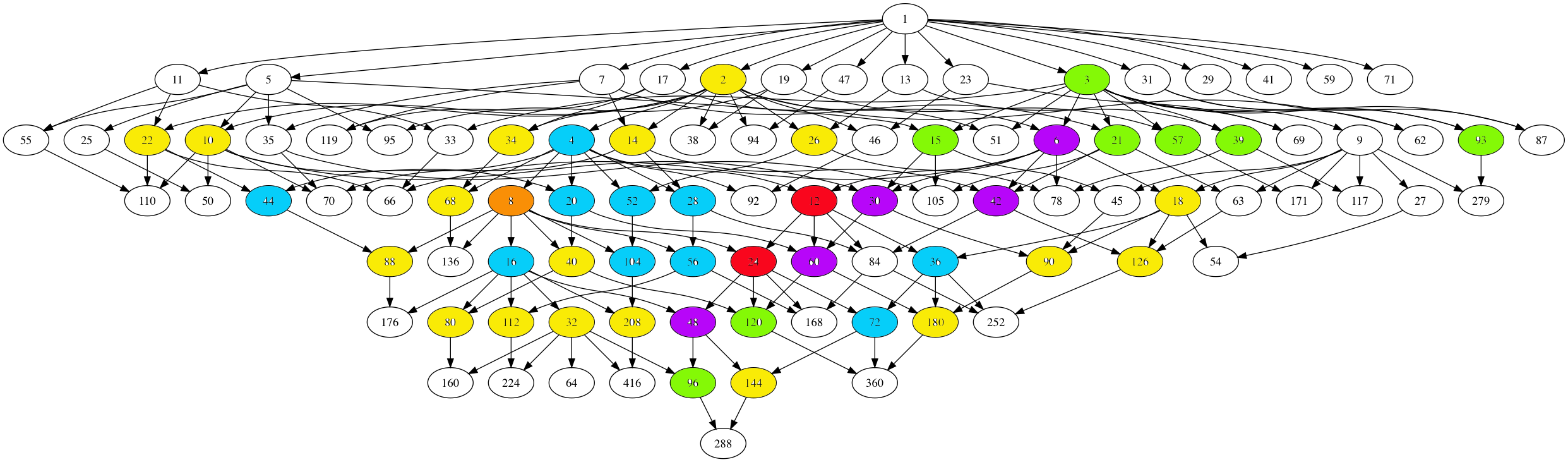
There are seven types of coloured numbers, each corresponding to number-lattices which have the same local structure in the moonshine picture, as in the previous post.

The white numbered lattices have no further edges in the picture.

The yellow number lattices (2,10,14,18,22,26,32,34,40,68,80,88,90,112,126,144,180,208 = 2M) have local structure

\[
\xymatrix{& \color{yellow}{2M} \ar@{-}[r] & M \frac{1}{2}} \]

The green number lattices (3,15,21,39,57,93,96,120 = 3M) have local structure

\[
\xymatrix{M \frac{1}{3} \ar@[red]@{-}[r] & \color{green}{3M} \ar@[red]@{-}[r] & M \frac{2}{3}} \]

The blue number lattices (4,16,20,28,36,44,52,56,72,104 = 4M) have as local structure

\[
\xymatrix{M \frac{1}{2} \ar@{-}[d] & & M \frac{1}{4} \ar@{-}[d] \\
2M \ar@{-}[r] & \color{blue}{4M} \ar@{-}[r] & 2M \frac{1}{2} \ar@{-}[d] \\
& & M \frac{3}{4}} \]

where the leftmost part is redundant as they are already included in the yellow-bit.

The purple number lattices (6,30,42,48,60 = 6M) have local structure

\[
\xymatrix{M \frac{1}{3} \ar@[red]@{-}[d] & 2M \frac{1}{3} & M \frac{1}{6} \ar@[red]@{-}[d] & \\
3M \ar@{-}[r] \ar@[red]@{-}[d] & \color{purple}{6M} \ar@{-}[r] \ar@[red]@{-}[u] \ar@[red]@{-}[d] & 3M \frac{1}{2} \ar@[red]@{-}[r] \ar@[red]@{-}[d] & M \frac{5}{6} \\
M \frac{2}{3} & 2M \frac{2}{3} & M \frac{1}{2} & } \]

where again the lefmost part is redundant, and I forgot to add the central part in the previous post… (updated now).

The unique brown number lattice 8 has local structure

\[
\xymatrix{& & 1 \frac{1}{4} \ar@{-}[d] & & 1 \frac{1}{8} \ar@{-}[d] & \\
& 1 \frac{1}{2} \ar@{-}[d] & 2 \frac{1}{2} \ar@{-}[r] \ar@{-}[d] & 1 \frac{3}{4} & 2 \frac{1}{4} \ar@{-}[r] & 1 \frac{5}{8} \\
1 \ar@{-}[r] & 2 \ar@{-}[r] & 4 \ar@{-}[r] & \color{brown}{8} \ar@{-}[r] & 4 \frac{1}{2} \ar@{-}[d] \ar@{-}[u] & \\
& & & 1 \frac{7}{8} \ar@{-}[r] & 2 \frac{3}{4} \ar@{-}[r] & 1 \frac{3}{8}} \]

The local structure in the two central red number lattices (not surprisingly 12 and 24) looks like the image in the previous post, but I have to add some ‘forgotten’ lattices.

That’ll have to wait…

Leave a Comment

a COLgo endgame

COL is a map-colouring game, attibuted to Colin Vout. COLgo is COL played with Go-stones on a go-board.

The two players, bLack (left) and white (right) take turns placing a stone of their colour on the board, but two stones of the same colour may not be next to each other.

The first player unable to make a legal move looses this game.

As is common in combinatorial game theory we do not specify which player has the move. There are $4$ different outcomes, the game is called:

– positive, if there is a winning strategy for Left (bLack),
– negative, if there is a winning strategy for Right (white),
– zero, if there is a winning strategy for the second-player,
– fuzzy, if there is a winning strategy for the first player.

Here’s an endgame problem: who wins this game?

Spoiler alert: solution below.

First we can exclude all spots which are dead, that is, are excluded for both players. Example, F11 is dead because it neighbors a black as well as a white stone, but F10 is alive as it can be played by white (Right).

If we remove all dead spots, we are left with 4 regions (the four extremal corners of the board) as well as 5 spots, 3 for white and 2 for black.

That is, the game reduces to this “sum”-game, in which a player chooses one of the regions and does a legal move in that component, or takes a stone of its own colour from the second row.

Next, we have to give a value to each of the region-games.

– the right-most game has value $0$ as the second player has a winning strategy by reflecting the first player’s move with respect to the central (dead) spot.

– the left-most game is equivalent to one black stone. Black can make two moves in the game, independent of the only move that white can make. So it has value $+1$.

– the sum-game of the two middle games has value zero. The second player can win by mirroring the first player’s move in the other component. This is called the Tweedledee-Tweedledum argument.

But then, the total value of the endgame position is

zero, so the first player to move looses the game!

Leave a Comment

Penrose tiles in Helsinki


(image credit: Steve’s travels & stuff)

A central street in Helsinki has been paved with Penrose tiles.


(image credit: Sattuman soittoa)

From a Finnish paper:

“The street could also be an object to mathematical awe. The stone under one’s feet is embroidered with some profound geometry, namely, Penrose tiling.

In 1974, a British mathematician Roger Penrose realised a plane could be fully covered with a few simple rules such that the pattern constantly changes. These kind of discontinuous patterns are interesting to mathematicians since the patterns can be used to solve other geometrical problems. Together, the tiles can randomly form patterns reminding a star or the Sun but they do not regularly recur in the tiling.

Similar features are found in the old Arabic ornaments. The tiling of the Central Street prom was selected by Yrjö Rossi.

If your kid stays put to stare at the tiling, they might have what they need in order to become a mathematician.”

(via Reddit/m)

Leave a Comment