Category: groups

The Leech lattice neighbour

Published March 23, 2021 by lievenlb

Here’s the upper part of Kneser‘s neighbourhood graph of the Niemeier lattices:

The Leech lattice has a unique neighbour, that is, among the $23$ remaining Niemeier lattices there is a unique one, $(A_1^{24})^+$ , sharing an index two sub-lattice with the Leech.

How would you try to construct $(A_1^{24})^+$ , an even unimodular lattice having the same roots as $A_1^{24}$ ?

The root lattice $A_1$ is $\sqrt{2} \mathbb{Z}$ . It has two roots $\pm \sqrt{2}$ , determinant $2$ , its dual lattice is $A_1^* = \tfrac{1}{\sqrt{2}} \mathbb{Z}$ and we have $A_1^*/A_1 \simeq C_2 \simeq \mathbb{F}_2$ .

Thus, $A_1^{24}= \sqrt{2} \mathbb{Z}^{\oplus 24}$ has $48$ roots, determinant $2^{24}$ , its dual lattice is $(A_1^{24})^* = \tfrac{1}{\sqrt{2}} \mathbb{Z}^{\oplus 24}$ and the quotient group $(A_1^{24})^*/A_1^{24}$ is $C_2^{24}$ isomorphic to the additive subgroup of $\mathbb{F}_2^{\oplus 24}$ .

A larger lattice $A_1^{24} \subseteq L$ of index $k$ gives for the dual lattices an extension $L^* \subseteq (A_1^{24})^*$ , also of index $k$ . If $L$ were unimodular, then the index has to be $2^{12}$ because we have the situation
$A_1^{24} \subseteq L = L^* \subseteq (A_1^{24})^*$
So, Kneser’s glue vectors form a $12$ -dimensional subspace $\mathcal{C}$ in $\mathbb{F}_2^{\oplus 24}$ , that is,
$L = \mathcal{C} \underset{\mathbb{F}_2}{\times} (A_1^{24})^* = \{ \tfrac{1}{\sqrt{2}} \vec{v} ~|~\vec{v} \in \mathbb{Z}^{\oplus 24},~v=\vec{v}~mod~2 \in \mathcal{C} \}$
Because $L = L^*$ , the linear code $\mathcal{C}$ must be self-dual meaning that $v.w = 0$ (in $\mathbb{F}_2$ ) for all $v,w \in \mathcal{C}$ . Further, we want that the roots of $A_1^{24}$ and $L$ are the same, so the minimal number of non-zero coordinates in $v \in \mathcal{C}$ must be $8$ .

That is, $\mathcal{C}$ must be a self-dual binary code of length $24$ with Hamming distance $8$ .

Marcel Golay (1902-1989) – Photo Credit

We now know that there is a unique such code, the (extended) binary Golay code, $\mathcal{C}_{24}$ , which has

one vector of weight $0$
$759$ vectors of weight $8$ (called ‘octads’)
$2576$ vectors of weight $12$ (called ‘dodecads’)
$759$ vectors of weight $16$
one vector of weight $24$

The $759$ octads form a Steiner system $S(5,8,24)$ (that is, for any $5$ -subset $S$ of the $24$ -coordinates there is a unique octad having its non-zero coordinates containing $S$ ).

Witt constructed a Steiner system $S(5,8,24)$ in his 1938 paper “Die $5$ -fach transitiven Gruppen von Mathieu”, so it is not unthinkable that he checked the subspace of $\mathbb{F}_2^{\oplus 24}$ spanned by his $759$ octads to be $12$ -dimensional and self-dual, thereby constructing the Niemeier-lattice $(A_1^{24})^+$ on that sunday in 1940.

John Conway classified all nine self-dual codes of length $24$ in which the weight
of every codeword is a multiple of $4$ . Each one of these codes $\mathcal{C}$ gives a Niemeier lattice $\mathcal{C} \underset{\mathbb{F}_2}{\times} (A_1^{24})^*$ , all but one of them having more roots than $A_1^{24}$ .

Vera Pless and Neil Sloan classified all $26$ binary self-dual codes of length $24$ .

Witt and his Niemeier lattices

Published March 19, 2021 by lievenlb

Sunday, January 28th 1940, Hamburg

Ernst Witt wants to get two papers out of his system because he knows he’ll have to enter the Wehrmacht in February.

The first one, “Spiegelungsgruppen und Aufzählung halbeinfacher Liescher Ringe”, contains his own treatment of the root systems of semisimple Lie algebras and their reflexion groups, following up on previous work by Killing, Cartan, Weyl, van der Waerden and Coxeter.

(Photo: Natascha Artin, Nikolausberg 1933): From left to right: Ernst Witt; Paul Bernays; Helene Weyl; Hermann Weyl; Joachim Weyl, Emil Artin; Emmy Noether; Ernst Knauf; unknown woman; Chiuntze Tsen; Erna Bannow (later became wife of Ernst Witt)

Important for our story is that this paper contains the result stating that integral lattices generated by norm 2 elements are direct sums of root systems of the simply laced Dynkin diagrans $A_n, D_n$ and $E_6,E_7$ or $E_8$ (Witt uses a slightly different notation).

In each case, Witt knows of course the number of roots and the determinant of the Gram matrix
$\begin{array}{c|cc} & \# \text{roots} & \text{determinant} \\ \hline A_n & n^2+n & n+1 \\ D_n & 2n^2-2n & 4 \\ E_6 & 72 & 3 \\ E_7 & 126 & 2 \\ E_8 & 240 & 1 \end{array}$
The second paper “Eine Identität zwischen Modulformen zweiten Grades” proves that there are just two positive definite even unimodular lattices (those in which every squared length is even, and which have one point per unit volume, that is, have determinant one) in dimension sixteen, $E_8 \oplus E_8$ and $D_{16}^+$ . Previously, Louis Mordell showed that the only unimodular even lattice in dimension $8$ is $E_8$ .

The connection with modular forms is via their theta series, listing the number of lattice points of each squared length
$\theta_L(q) = \sum_{m=0}^{\infty} \#\{ \lambda \in L : (\lambda,\lambda)=m \} q^{m}$
which is a modular form of weight $n/2$ ( $n$ being the dimension which must be divisible by $8$ ) in case $L$ is a positive definitive even unimodular lattice.

The algebra of all modular forms is generated by the Eisenstein series $E_2$ and $E_3$ of weights $4$ and $6$ , so in dimension $8$ we have just one possible theta series
$\theta_L(q) = E_2^2 = 1+480 q^2+ 61920 q^4+ 1050240 q^6+ \dots$

It is interesting to read Witt’s proof of his main result (Satz 3) in which he explains how he constructed the possible even unimodular lattices in dimension $16$ .

He knows that the sublattice of $L$ generated by the $480$ norm two elements must be a direct sum of root lattices. His knowledge of the number of roots in each case tells him there are only two possibilities
$E_8 \oplus E_8 \qquad \text{and} \qquad D_{16}$
The determinant of the Gram matrix of $E_8 \oplus E_8$ is one, so this one is already unimodular. The remaining possibility
$D_{16} = \{ (x_1,\dots,x_{16}) \in \mathbb{Z}^{16}~|~x_1+ \dots + x_{16} \in 2 \mathbb{Z} \}$
has determinant $4$ so he needs to add further lattice points (necessarily contained in the dual lattice $D_{16}^*$ ) to get it unimodular. He knows the coset representatives of $D_{16}^*/D_{16}$ :
$\begin{cases} [0]=(0, \dots,0) &~\text{of norm $0$} \\ [1]=(\tfrac{1}{2},\dots,\tfrac{1}{2}) &~\text{of norm $4$} \\ [2]=(0,\dots,0,1) &~\text{of norm $1$} \\ [3]=(\tfrac{1}{2},\dots,\tfrac{1}{2},-\tfrac{1}{2}) &~\text{of norm $4$} \end{cases}$
and he verifies that the determinant of $D_{16}^+=D_{16}+([1]+D_{16})$ is indeed one (btw. adding coset $[3]$ gives an isomorphic lattice). Witt calls this procedure to arrive at the correct lattices forced (‘zwangslaufig’).

So, how do you think Witt would go about finding even unimodular lattices in dimension $24$ ?

To me it is clear that he would start with a direct sum of root lattices whose dimensions add up to $24$ , compute the determinant of the Gram matrix and, if necessary, add coset classes to arrive at a unimodular lattice.

Today we would call this procedure ‘adding glue’, after Martin Kneser, who formalised this procedure in 1967.

On January 28th 1940, Witt writes that he found more than $10$ different classes of even unimodular lattices in dimension $24$ (without giving any details) and mentioned that the determination of the total number of such lattices will not be entirely trivial (‘scheint nicht ganz leicht zu sein’).

The complete classification of all $24$ even unimodular lattices in dimension $24$ was achieved by Hans Volker Niemeier in his 1968 Ph.D. thesis “Definite quadratische Formen der Dimension 24 und Diskriminante 1”, under the direction of Martin Kneser. Naturally, these lattices are now known as the Niemeier lattices.

Which of the Niemeier lattices were known to Witt in 1940?

There are three obvious certainties: $E_8 \oplus E_8 \oplus E_8$ , $E_8 \oplus D_{16}^+$ (both already unimodular, the second by Witt’s work) and $D_{24}^+$ with a construction analogous to the one of $D_{16}^+$ .

To make an educated guess about the remaining Witt-Niemeier lattices we can do two things:

use our knowledge of Niemeier lattices to figure out which of these Witt was most likely to stumble upon, and
imagine how he would adapt his modular form approach in dimension $16$ to dimension $24$ .

Here’s Kneser’s neighbourhood graph of the Niemeier lattices. Its vertices are the $24$ Niemeiers and there’s an edge between $L$ and $M$ whenever the intersection $L \cap M$ is of index $2$ in both $L$ and $M$ . In this case, $L$ and $M$ are called neighbours.

Although the theory of neighbours was not known to Witt, the graph may give an indication of how likely it is to dig up a new Niemeier lattice by poking into an already discovered one.
The three certainties are the three lattices at the bottom of the neighborhood graph, making it more likely for the lattices in the lower region to be among Witt’s list.

For the other approach, the space of modular forms of weight $12$ is two dimensional, with a basis formed by the series
$\begin{cases} E_6(q) = 1 + \tfrac{65520}{691}(q+2049 q^2 + 177148 q^3+4196353q^4+\dots \\ \Delta(q) = q-24 q^2+252q^3-1472q^4+ \dots \end{cases}$

If you are at all with me, Witt would start with a lattice $R$ which is a direct sum of root lattices, so he would know the number of its roots (the norm $2$ vectors in $R$ ), let’s call this number $r$ . Now, he wants to construct an even unimodular lattice $L$ containing $R$ , so the theta series of both $L$ and $R$ must start off with $1 + r q^2 + \dots$ . But, then he knows
$\theta_L(q) = E_6(q) + (r-\frac{65520}{691})\Delta(q)$
and comparing coefficients of $\theta_L(q)$ with those of $\theta_R(q)$ will give him an idea what extra vectors he has to throw in.

If we’re generous to Witt (and frankly, why shouldn’t we), we may believe that he used his vast knowledge of Steiner systems (a few years earlier he wrote the definite paper on the Mathieu groups, and a paper on Steiner systems) to construct in this way the lattices $(A_1^{24})^+$ and $(A_2^{12})^+$ .

The ‘glue’ for $(A_1^{24})^+$ is coming from the extended binary Golay code, which itself uses the Steiner system $S(5,8,24)$ . $(A_2^{12})^+$ is constructed using the extended ternary Golay code, based on the Steiner system $S(5,6,12)$ .

The one thing that would never have crossed his mind that sunday in 1940 was to explore the possibility of an even unimodular 24-dimensional lattice $\Lambda$ without any roots!

One with $r=0$ , and thus with a theta series starting off as
$\theta_{\Lambda}(q) = 1 + 196560 q^4 + 16773120 q^6 + \dots$
No, he did not find the Leech lattice that day.

If he would have stumbled upon it, it would have simply blown his mind.

It would have been so much against all his experiences and intuitions that he would have dropped everything on the spot to write a paper about it, or at least, he would have mentioned in his ‘more than $10$ lattices’-claim that, surprisingly, one of them was an even unimodular lattice without any roots.

de Bruijn’s pentagrids (2)

Published March 17, 2021 by lievenlb

Last time we’ve seen that de Bruijn’s pentagrids determined the vertices of Penrose’s P3-aperiodic tilings.

These vertices can also be obtained by projecting a window of the standard hypercubic lattice $\mathbb{Z}^5$ by the cut-and-project-method.

We’ll bring in representation theory by forcing this projection to be compatible with a $D_5$ -subgroup of the symmetries of $\mathbb{Z}^5$ , which explains why Penrose tilings have a local $D_5$ -symmetry.

The symmetry group of the standard $n$ -dimensional hypercubic lattice
$\mathbb{Z} \vec{e}_1 + \dots + \mathbb{Z} \vec{e}_n \subset \mathbb{R}^n$
is the hyperoctahedral group of all signed $n \times n$ permutation matrices
$B_n = C_2^n \rtimes S_n$
in which all $n$ -permutations $S_n$ act on the group $C_2^n = \{ 1,-1 \}^n$ of all signs. The signed permutation $n \times n$ matrix corresponding to an element $(\vec{a},\pi) \in B_n$ is given by
$T_{ij} = T(\vec{a},\pi)_{ij} = a_j \delta_{i,\pi(j)}$
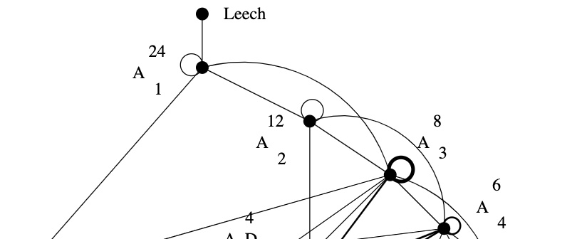
The represenation theory of $B_n$ was worked out in 1930 by the British mathematician and clergyman Alfred Young

We want to do explicit calculations in

$B_n$ using a computational system such as GAP, so it is best to describe

$B_n$ as a permutation subgroup of

$S_{2n}$ via the morphism

$\tau((\vec{a},\pi))(k) = \begin{cases} \pi(k)+n \delta_{-1,a_k}~\text{if $1 \leq k \leq n$} \\ \pi(k-n)+n(1-\delta_{-1,a_{k-n}})~\text{if $n+1 \leq k \leq 2n$} \end{cases}$
the image is generated by the permutations

$\begin{cases} \alpha = (1,2)(n+1,n+2), \\ \beta=(1,2,\dots,n)(n+1,n+2,\dots,2n), \\ \gamma=(n,2n) \end{cases}$
and to a permutation

$\sigma \in \tau(B_n) \subset S_{2n}$ we assign the signed permutation

$n \times n$ matrix

$T_{\sigma}=T(\tau^{-1}(\pi))$ .

We use GAP to set up $B_5$ from these generators and determine all its conjugacy classes of subgroups. It turns out that $B_5$ has no less than $953$ different conjugacy classes of subgroups.

gap> B5:=Group((1,2)(6,7),(1,2,3,4,5)(6,7,8,9,10),(5,10));
Group([ (1,2)(6,7), (1,2,3,4,5)(6,7,8,9,10), (5,10) ])
gap> Size(B5);
3840
gap> C:=ConjugacyClassesSubgroups(B5);;
gap> Length(C);
953

But we are only interested in the subgroups isomorphic to $D_5$ . So, first we make a sublist of all conjugacy classes of subgroups of order $10$ , and then we go through this list one-by-one and look for an explicit isomorphism between $D_5 = \langle x,y~|~x^5=e=y^2,~xyx=y \rangle$ and a representative of the class (or get a ‘fail’ is this subgroup is not isomorphic to $D_5$ ).

gap> C10:=Filtered(C,x->Size(Representative(x))=10);;
gap> Length(C10);
3
gap> s10:=List(C10,Representative);
[ Group([ (2,5)(3,4)(7,10)(8,9), (1,5,4,3,2)(6,10,9,8,7) ]),
Group([ (1,6)(2,5)(3,4)(7,10)(8,9), (1,10,9,3,2)(4,8,7,6,5) ]),
Group([ (1,6)(2,7)(3,8)(4,9)(5,10), (1,2,8,4,10)(3,9,5,6,7) ]) ]
gap> D:=DihedralGroup(10); gap> IsomorphismGroups(D,s10[1]);
[ f1, f2 ] -> [ (2,5)(3,4)(7,10)(8,9), (1,5,4,3,2)(6,10,9,8,7) ]
gap> IsomorphismGroups(D,s10[2]);
[ f1, f2 ] -> [ (1,6)(2,5)(3,4)(7,10)(8,9), (1,10,9,3,2)(4,8,7,6,5) ]
gap> IsomorphismGroups(D,s10[3]);
fail
gap> IsCyclic(s10[3]);
true

Of the three (conjugacy classes of) subgroups of order $10$ , two are isomorphic to $D_5$ , and the third one to $C_{10}$ . Next, we have to transform the generating permutations into signed $5 \times 5$ permutation matrices using the bijection $\tau^{-1}$ .
$\begin{array}{c|c} \sigma & (\vec{a},\pi) \\ \hline (2,5)(3,4)(7,10)(8,9) & ((1,1,1,1,1),(2,5)(3,4)) \\ (1,5,4,3,2)(6,10,9,8,7) & ((1,1,1,1,1)(1,5,4,3,2)) \\ (1,6)(2,5)(3,4)(7,10)(8,9) & ((-1,1,1,1,1),(2,5)(3,4)) \\ (1,10,9,3,2)(4,8,7,6,5) & ((-1,1,1,-1,1),(1,5,4,3,2)) \end{array}$
giving the signed permutation matrices
$\begin{array}{c|cc} & x & y \\ \hline A & \begin{bmatrix} 0 & 1 & 0 & 0 & 0 \\ 0 & 0 & 1 & 0 & 0 \\ 0 & 0 & 0 & 1 & 0 \\ 0 & 0 & 0 & 0 & 1 \\ 1 & 0 & 0 & 0 & 0 \end{bmatrix} & \begin{bmatrix} 1 & 0 & 0 & 0 & 0 \\ 0 & 0 & 0 & 0 & 1 \\ 0 & 0 & 0 & 1 & 0 \\ 0 & 0 & 1 & 0 & 0 \\ 0 & 1 & 0 & 0 & 0 \end{bmatrix} \\ \hline B & \begin{bmatrix} 0 & 1 & 0 & 0 & 0 \\ 0 & 0 & 1 & 0 & 0 \\ 0 & 0 & 0 & -1 & 0 \\ 0 & 0 & 0 & 0 & 1 \\ -1 & 0 & 0 & 0 & 0 \end{bmatrix} & \begin{bmatrix} -1 & 0 & 0 & 0 & 0 \\ 0 & 0 & 0 & 0 & 1 \\ 0 & 0 & 0 & 1 & 0 \\ 0 & 0 & 1 & 0 & 0 \\ 0 & 1 & 0 & 0 & 0 \end{bmatrix} \end{array}$
$D_5$ has $4$ conjugacy classes with representatives $e,y,x$ and $x^2$ . the
character table of $D_5$ is
$\begin{array}{c|cccc} & (1) & (2) & (2) & (5) \\ & 1_a & 5_1 & 5_2 & 2_a \\ D_5 & e & x & x^2 & y \\ \hline T & 1 & 1 & 1 & 1 \\ V & 1 & 1 & 1 & -1 \\ W_1 & 2 & \tfrac{-1+ \sqrt{5}}{2} & \tfrac{-1 -\sqrt{5}}{2} & 0 \\ W_2 & 2 & \tfrac{-1 -\sqrt{5}}{2} & \tfrac{-1+\sqrt{5}}{2} & 0 \end{array}$
Using the signed permutation matrices it is easy to determine the characters of the $5$ -dimensional representations $A$ and $B$
$\begin{array}{c|cccc} D_5 & e & x & x^2 & y \\ \hline A & 5 & 0 & 0 & 1 \\ B & 5 & 0 & 0 & -1 \end{array}$
decomosing into $D_5$ -irreducibles as
$A \simeq T \oplus W_1 \oplus W_2 \quad \text{and} \quad B \simeq V \oplus W_1 \oplus W_2$
Representation $A$ realises $D_5$ as a rotation symmetry group of the hypercube lattice $\mathbb{Z}^5$ in $\mathbb{R}^5$ , and next we have to find a $D_5$ -projection $\mathbb{R}^5=A \rightarrow W_1 = \mathbb{R}^2$ .

As a complex representation $A \downarrow_{C_5}$ decomposes as a direct sum of $1$ -dimensional representations
$A \downarrow_{C_5} = V_1 \oplus V_{\zeta} \oplus V_{\zeta^2} \oplus V_{\zeta^3} \oplus V_{\zeta^4}$
where $\zeta = e^{2 \pi i /5}$ and where the action of $x$ on $V_{\zeta^i}=\mathbb{C} v_i$ is given by $x.v_i = \zeta^i v_i$ . The $x$ -eigenvectors in $\mathbb{C}^5$ are
$\begin{cases} v_0 = (1,1,1,1,1) \\ v_1 = (1,\zeta,\zeta^2,\zeta^3,\zeta^4) \\ v_2 =(1,\zeta^2,\zeta^4,\zeta,\zeta^3) \\ v_3 = (1,\zeta^3,\zeta,\zeta^4,\zeta^2) \\ v_4 = (1,\zeta^4,\zeta^3,\zeta^2,\zeta) \end{cases}$
The action of $y$ on these vectors is given by $y.v_i = v_{5-i}$ because
$x.(y.v_i) = (xy).v_i=(yx^{-1}).v_i=y.(x^{-1}.v_i) = y.(\zeta^{-i} v_i) = \zeta^{-1} (y.v_i)$
and therefore $y.v_i$ is an $x$ -eigenvector with eigenvalue $\zeta^{5-i}$ . As a complex $D_5$ -representation, the factors of $A$ are therefore
$T = \mathbb{C} v_0, \quad W_1 = \mathbb{C} v_1 + \mathbb{C} v_4, \quad \text{and} \quad W_2 = \mathbb{C} v_2 + \mathbb{C} v_3$
But we want to consider $A$ as a real representation. As $\zeta^j = cos(\tfrac{2 \pi j}{5})+i~sin(\tfrac{2 \pi j}{5}) = c_j + i s_j$ hebben we can take the vectors in $\mathbb{R}^5$
$\begin{cases} \frac{1}{2}(v_1+v_4) = (1,c_1,c_2,c_3,c_4)= u_1 \\ -\frac{1}{2}i(v_1-v_4) = (0,s_1,s_2,s_3,s_4) = u_2 \\ \frac{1}{2}(v_2+v_3) = (1,c_2,c_4,c1,c3)= w_1 \\ -\frac{1}{2}i(v_2-v_3) = (0,s_2,s_4,s_1,s_3)= w_2 \end{cases}$
and $A$ decomposes as a real $D_5$ -representation with
$T = \mathbb{R} v_0, \quad W_1 = \mathbb{R} u_1 + \mathbb{R} u_2, \quad \text{and} \quad W_2 = \mathbb{R} w_1 + \mathbb{R} w_2$
and if we identify $\mathbb{C}$ with $\mathbb{R}^2$ via $z \leftrightarrow (Re(z),Im(z))$ we can describe the $D_5$ -projection morphism $\pi_{W_1}~:~\mathbb{R}^5=A \rightarrow W_1=\mathbb{R}^2$ via
$(y_0,y_1,y_2,y_3,y_4) \mapsto y_0+y_1 \zeta + y_2 \zeta^2 + y_3 \zeta^3 + y_4 \zeta^4 = \sum_{i=0}^4 y_i (c_i,s_i)$
Note also that $W_1$ is the orthogonal complement of $T \oplus W_2$ , so is equal to the linear subspace in $\mathbb{R}^5$ determined by the three linear equations
$\begin{cases} \sum_{i=0}^4 x_i = 0 \\ \sum_{i=0}^4 c_{2i} x_i = 0 \\ \sum_{i=0}^4 s_{2i} x_i = 0 \end{cases}$

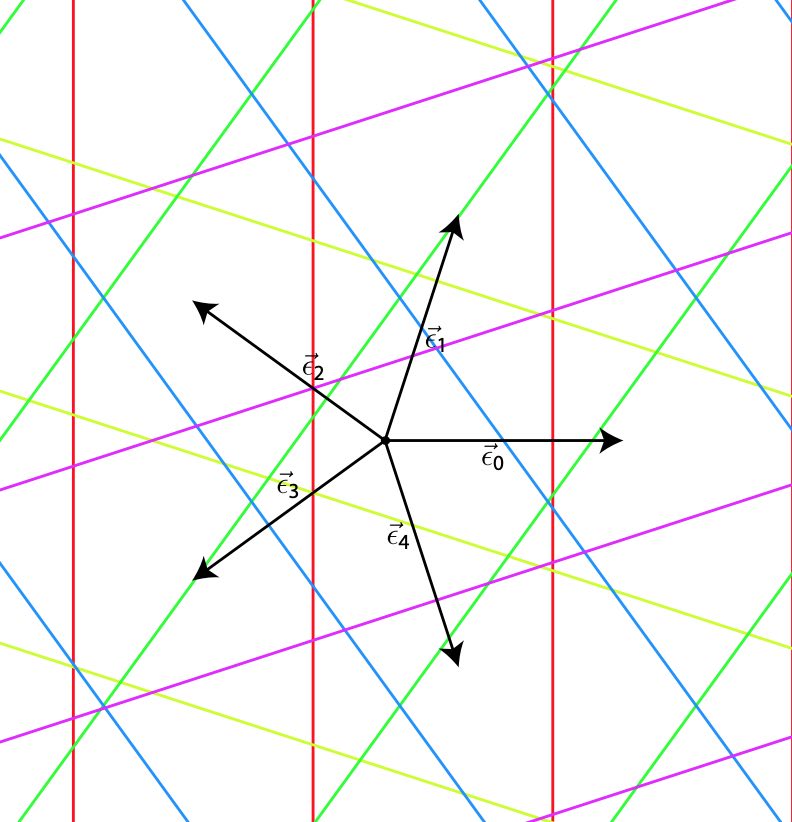
Okay, now take the Rhombic tiling corresponding to the regular pentagrid defined by $\gamma_0, \dots, \gamma_4$ satisfying $\sum_{i=0}^4 \gamma_i = 0$ . Let $\vec{k}=(k_0,\dots,k_4) \in \mathbb{Z}^5$ and define the open hypercube $H_{\vec{k}}$ corresponding to $\vec{k}$ as the set of points
$(x_0,\dots,x_4) \in \mathbb{R}^5~:~\forall 0 \leq i \leq 4~:~k_i – 1 < x_i < k_i$ From the vector $\vec{\gamma} = (\gamma_0,\dots,\gamma_4)$ determining the Rhombic tiling we define the $2$ -dimensional plane $P_{\vec{\gamma}}$ in $\mathbb{R}^5$ given by the equations $\begin{cases} \sum_{i=0}^4 x_i = 0 \\ \sum_{i=0}^4 c_{2i} (x_i - \gamma_i) = 0 \\ \sum_{i=0}^4 s_{2i} (x_i - \gamma_i) = 0 \end{cases}$ The point being that $P_{\vec{\gamma}}$ is the linear plane $W_1$ in $\mathbb{R}^5$ translated over the vector $\vec{\gamma}$ , so it is parallel to $W_1$ . Here's the punchline:

de Bruijn’s theorem: The vertices of the Rhombic tiling produced by the regular pentagrid with parameters $\vec{\gamma}=(\gamma_0,\dots,\gamma_4)$ are the points
$\sum_{i=0}^4 k_i (c_i,s_i)$
with $\vec{k}=(k_0,\dots,k_4) \in \mathbb{Z}^5$ such that $H_{\vec{k}} \cap P_{\vec{\gamma}} \not= \emptyset$ .

To see this, let $\vec{x} = (x_0,\dots,x_4) \in P_{\vec{\gamma}}$ , then $\vec{x}-\vec{\gamma} \in W_1$ , but then there is a vector $\vec{y} \in \mathbb{R}^2$ such that
$x_j – \gamma_j = \vec{y}.\vec{v}_j \quad \forall~0 \leq j \leq 4$
But then, with $k_j=\lceil \vec{y}.\vec{v}_j + \gamma_j \rceil$ we have that $\vec{x} \in H_{\vec{k}}$ and we note that $V(\vec{y}) = \sum_{i=0}^4 k_i \vec{v}_i$ is a vetex of the Rhombic tiling associated to the regular pentagrid parameters $\vec{\gamma}=(\gamma_0,\dots,\gamma_4)$ .

Here we used regularity of the pentagrid in order to have that $k_j=\vec{y}.\vec{v}_j + \gamma_j$ can happen for at most two $j$ ’s, so we can manage to vary $\vec{y}$ a little in order to have $\vec{x}$ in the open hypercube.

Here’s what we did so far: we have identified $D_5$ as a group of rotations in $\mathbb{R}^5$ , preserving the hypercube-lattice $\mathbb{Z}^5$ in $\mathbb{R}^5$ . If the $2$ -plane $P_{\vec{\gamma}}$ is left stable under these rotations, then because rotations preserve distances, also the subset of lattice-points
$S_{\vec{\gamma}} = \{ (k_0,\dots,k_4)~|~H_{\vec{k}} \cap P_{\vec{\gamma}} \not= \emptyset \} \subset \mathbb{Z}^5$
is left stable under the $D_5$ -action. But, because the map
$(k_0,\dots,k_4) \mapsto \sum_{i=0}^4 k_i (c_i,s_i)$
is the $D_5$ -projection map $\pi : A \rightarrow W_1$ , the vertices of the associated Rhombic tiling must be stable under the $D_5$ -action on $W_1$ , meaning that the Rhombic tiling should have a global $D_5$ -symmetry.

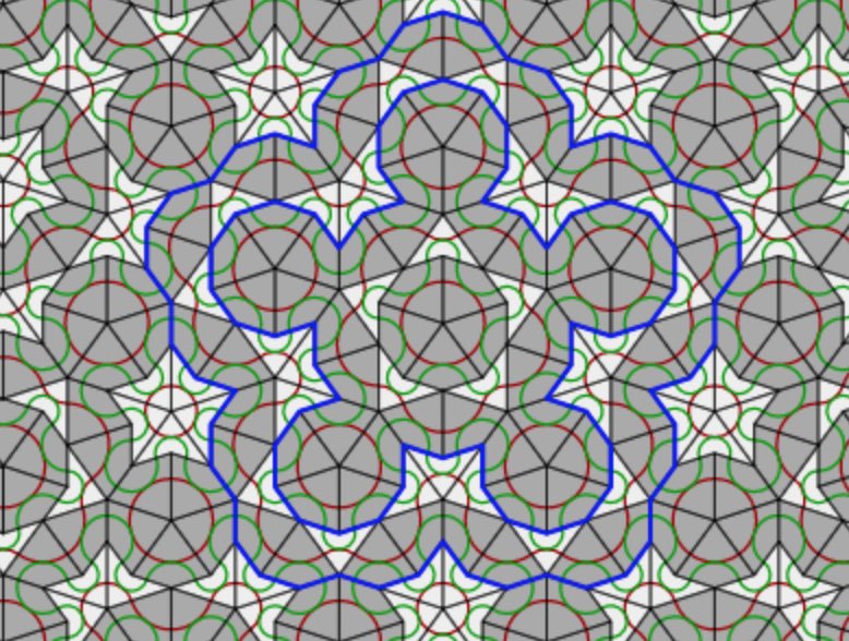
Sadly, the only plane $P_{\vec{\gamma}}$ left stable under all rotations of $D_5$ is when $\vec{\gamma} = \vec{0}$ , which is an exceptionally singular pentagrid. If we project this situation we do indeed get an image with global $D_5$ -symmetry

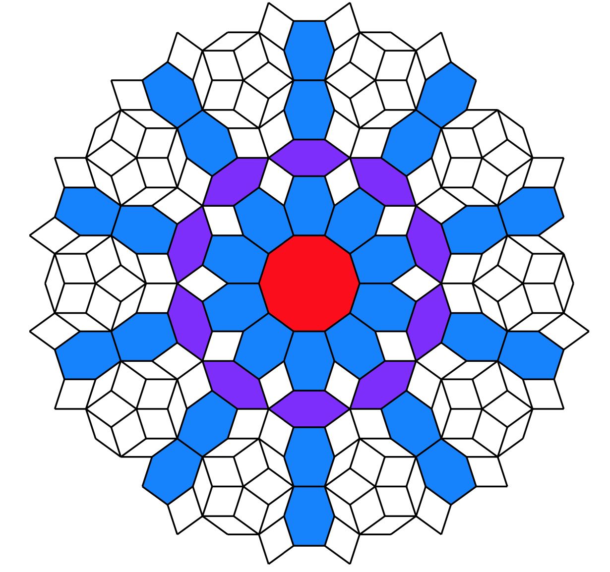
but it is not a Rhombic tiling. What’s going on?

Because this post is already dragging on for far too long (TL;DR), we’ll save the investigation of projections of singular pentagrids, how they differ from the regular situation, and how they determine multiple Rhombic tilings, for another time.