Category: games

can -oids save group-theory 101?

Published February 15, 2009 by lievenlb

Two questions from my last group-theory 101 exam:

(a) : What are the Jordan-Holder components of the Abelian group $\mathbb{Z}/20 \mathbb{Z} $?

(b) : Determine the number of order 7 elements in a simple group of order 168.

Give these to any group of working mathematicians, and, I guess all of them will solve (a), whereas the number of correct solutions to (b) will be (substantially) smaller.

Guess what? All(!) my students solved (b) correctly, whereas almost none of them had anything sensible to say about (a). A partial explanation is that they had more drill-exercises applying the Sylow-theorems than ones concerning the Jordan-Holder theorem.

A more fundamental explanation is that (b) has to do with sub-structures whereas (a) concerns quotients. Over the years I’ve tried numerous methods to convey the quotient-idea : putting things in bags, dividing a big group-table into smaller squares, additional lessons on relations, counting modulo numbers … No method appears to have an effect, lasting until the examination.

At the moment I’m seriously considering to rewrite the entire course, ditching quotients and using them only in disguise via groupoids. Before you start bombarding me with comments, I’m well aware of the problems inherent in this approach.

Before you do groupoids, students have to know some basic category theory. But that’s ok with me. Since last year it has been decided that I should sacrifice the first three weeks of the course telling students the basics of sets, maps and relations. After this, the formal definition of a category will appear more natural to them than the definition of a group, not? Besides, most puzzle-problems I use to introduce groups are actually examples of groupoids…

But then, what are the main theorems on finite groupoids? Well, I can see the groupoid cardinality result, giving you in one stroke Lagrange’s theorem as well as the orbit-counting method. From this one can then prove the remaining classical group-results such as Cauchy and the Sylows, but perhaps there are more elegant approaches?

Have you seen a first-year group-theory course starting off with groupoids? Do you know an elegant way to prove a classical group-result using groupoids?

2 Comments

On2 : extending Lenstra’s list

Published January 27, 2009 by lievenlb

We have seen that John Conway defined a nim-addition and nim-multiplication on the ordinal numbers in such a way that the subfield $[\omega^{\omega^{\omega}}] \simeq \overline{\mathbb{F}}_2 $ is the algebraic closure of the field on two elements. We’ve also seen how to do actual calculations in that field provided we can determine the mystery elements $\alpha_p $, which are the smallest ordinals not being a p-th power of ordinals lesser than $[\omega^{\omega^{k-1}}] $ if $p $ is the $k+1 $-th prime number.

Hendrik Lenstra came up with an effective method to compute these elements $\alpha_p $ requiring a few computations in certain finite fields. I’ll give a rundown of his method and refer to his 1977-paper “On the algebraic closure of two” for full details.

For any ordinal $\alpha < \omega^{\omega^{\omega}} $ define its degree $d(\alpha) $ to be the degree of minimal polynomial for $\alpha $ over $\mathbb{F}_2 = [2] $ and for each prime number $p $ let $f(p) $ be the smallest number $h $ such that $p $ is a divisor of $2^h-1 $ (clearly $f(p) $ is a divisor of $p-1 $).

In the previous post we have already defined ordinals $\kappa_{p^k}=[\omega^{\omega^{k-1}.p^{n-1}}] $ for prime-power indices, but we now need to extend this definition to allow for all indices. So. let $h $ be a natural number, $p $ the smallest prime number dividing $h $ and $q $ the highest power of $p $ dividing $h $. Let $g=[h/q] $, then Lenstra defines

$\kappa_h = \begin{cases} \kappa_q~\text{if q divides}~d(\kappa_q)~\text{ and} \\ \kappa_g + \kappa_q = [\kappa_g + \kappa_q]~\text{otherwise} \end{cases} $

With these notations, the main result asserts the existence of natural numbers $m,m’ $ such that

$\alpha_p = [\kappa_{f(p)} + m] = [\kappa_{f(p)}] + m’ $

Now, assume by induction that we have already determined the mystery numbers $\alpha_r $ for all odd primes $r < p $, then by teh argument of last time we can effectively compute in the field $[\kappa_p] $. In particular, we can compute for every element its multiplicative order $ord(\beta) $ and therefore also its degree $d(\beta) $ which has to be the smallest number $h $ such that $ord(\beta) $ divides $[2^h-1] $.

Then, by the main result we only have to determine the smallest number m such that $\beta = [\kappa_{f(p)} +m] $ is not a p-th power in $\kappa_p $ which is equivalent to the condition that

$\beta^{(2^{d(\beta)}-1)/p} \not= 1 $ if $p $ divides $[2^{d(\beta)}-1] $

All these conditions can be verified within suitable finite fields and hence are effective. In this manner, Lenstra could extend Conway’s calculations (probably using a home-made finite field program running on a slow 1977 machine) :

[tex]\begin{array}{c|c|c} p & f(p) & \alpha_p \\ \hline 3 & 2 & [2] \\ 5 & 4 & [4] \\ 7 & 3 & [\omega]+1 \\ 11 & 10 & [\omega^{\omega}]+1 \\ 13 & 12 & [\omega]+4 \\ 17 & 8 & [16] \\ 19 & 18 & [\omega^3]+4 \\ 23 & 11 & [\omega^{\omega^3}]+1 \\ 29 & 28 & [\omega^{\omega^2}]+4 \\ 31 & 5 & [\omega^{\omega}]+1 \\ 37 & 36 & [\omega^3]+4 \\ 41 & 20 & [\omega^{\omega}]+1 \\ 43 & 14 & [\omega^{\omega^2}]+ 1 \end{array}[/tex]

Right, so let’s try the case $p=47 $. To begin, $f(47)=23 $ whence we have to determine the smallest field containg $\kappa_{23} $. By induction (Lenstra’s tabel) we know already that

$\kappa_{23}^{23} = \kappa_{11} + 1 = [\omega^{\omega^3}]+1 $ and $\kappa_{11}^{11} = \kappa_5 + 1 = [\omega^{\omega}]+1 $ and $\kappa_5^5=[4] $

Because the smallest field containg $4 $ is $[16]=\mathbb{F}_{2^4} $ we have that $\mathbb{F}_2(4,\kappa_5,\kappa_{11}) \simeq \mathbb{F}_{2^{220}} $. We can construct this finite field, together with a generator $a $ of its multiplicative group in Sage via

sage: f1.< a >=GF(2^220)

In this field we have to pinpoint the elements $4,\kappa_5 $ and $\kappa_{11} $. As $4 $ has order $15 $ in $\mathbb{F}_{2^4} $ we know that $\kappa_5 $ has order $75 $. Hence we can take $\kappa_5 = a^{(2^{220}-1)/75} $ and then $4=\kappa_5^5 $.

If we denote $\kappa_5 $ by x5 we can obtain $\kappa_{11} $ as x11 by the following sage-commands

sage: c=x5+1

sage: x11=c.nth_root(11)

It takes about 7 minutes to find x11 on a 2.4 GHz MacBook. Next, we have to set up the field extension determined by $\kappa_{23} $ (which we will call x in sage). This is done as follows

sage: p1.=PolynomialRing(f1)


sage: f=x^23-x11-1

sage: F2=f1.extension(f,'u')

The MacBook needed 8 minutes to set up this field which is isomorphic to $\mathbb{F}_{2^{5060}} $. The relevant number is therefore $n=\frac{2^{5060}-1}{47} $ which is the gruesome

34648162040462867047623719793206539850507437636617898959901744136581<br/>
259144476645069239839415478030722644334257066691823210120548345667203443<br/>
317743531975748823386990680394012962375061822291120459167399032726669613
<br/>
442804392429947890878007964213600720766879334103454250982141991553270171

938532417844211304203805934829097913753132491802446697429102630902307815

301045433019807776921086247690468136447620036910689177286910624860871748

150613285530830034500671245400628768674394130880959338197158054296625733

206509650361461537510912269982522844517989399782602216622257291361930850

885916974186835958466930689748400561295128553674118498999873244045842040

080195019701984054428846798610542372150816780493166669821114184374697446

637066566831036116390063418916814141753876530004881539570659100352197393

997895251223633176404672792711603439161147155163219282934597310848529360

118189507461132290706604796116111868096099527077437183219418195396666836

014856037176421475300935193266597196833361131333604528218621261753883518

667866835204501888103795022437662796445008236823338104580840186181111557

498232520943552183185687638366809541685702608288630073248626226874916669

186372183233071573318563658579214650042598011275864591248749957431967297

975078011358342282941831582626985121760847852546207377440873367589369439

085660784239080183415569559585998884824991911321095149718147110882474280

968166266224151511519773175933506503369761671964823112231808283557885030

984081329986188655169245595411930535264918359325712373064120338963742590

76555755141425

Remains ‘only’ to take x,x+1,etc. to the n-th power and verify which is the first to be unequal to 1. For this it is best to implement the usual powering trick (via digital expression of the exponent) in the field F2, something like

sage: def power(e,n): ...: le=n.bits() ...: v=n.digits() ...: mn=F2(e) ...: out=F2(1) ...: i=0 ...: while i< le : ...: if v[i]==1 : out=F2(out_mn) ...: m=F2(mn_mn) ...: mn=F2(m) ...: i=i+1 ...: return(out) ...:

then it takes about 20 seconds to verify that power(x,n)=1 but that power(x+1,n) is NOT! That is, we just checked that $\alpha_{47}=\kappa_{11}+1 $.

It turns out that 47 is the hardest nut to crack, the following primes are easier. Here’s the data (if I didn’t make mistakes…)

[tex]\begin{array}{c|c|c} p & f(p) & \alpha_p \\ \hline 47 & 23 & [\omega^{\omega^{7}}]+1 \\ 53 & 52 & [\omega^{\omega^4}]+1 \\ 59 & 58 & [\omega^{\omega^8}]+1 \\ 61 & 60 & [\omega^{\omega}]+[\omega] \\ 67 & 66 & [\omega^{\omega^3}]+[\omega] \end{array}[/tex]

It seems that Magma is substantially better at finite field arithmetic, so if you are lucky enough to have it you’ll have no problem finding $\alpha_p $ for all primes less than 100 by the end of the day. If you do, please drop a comment with the results…

On2 : Conway’s nim-arithmetics

Published January 26, 2009 by lievenlb

Last time we did recall Cantor’s addition and multiplication on ordinal numbers. Note that we can identify an ordinal number $\alpha $ with (the order type of) the set of all strictly smaller ordinals, that is, $\alpha = { \alpha’~:~\alpha’ < \alpha } $. Given two ordinals $\alpha $ and $\beta $ we will denote their Cantor-sums and products as $[ \alpha + \beta] $ and $[\alpha . \beta] $.

The reason for these square brackets is that John Conway constructed a well behaved nim-addition and nim-multiplication on all ordinals $\mathbf{On}_2 $ by imposing the ‘simplest’ rules which make $\mathbf{On}_2 $ into a field. By this we mean that, in order to define the addition $\alpha + \beta $ we must have constructed before all sums $\alpha’ + \beta $ and $\alpha + \beta’ $ with $\alpha’ < \alpha $ and $\beta’ < \beta $. If + is going to be a well-defined addition on $\mathbf{On}_2 $ clearly $\alpha + \beta $ cannot be equal to one of these previously constructed sums and the ‘simplicity rule’ asserts that we should take $\alpha+\beta $ the least ordinal different from all these sums $\alpha’+\beta $ and $\alpha+\beta’ $. In symbols, we define

$\alpha+ \beta = \mathbf{mex} { \alpha’+\beta,\alpha+ \beta’~|~\alpha’ < \alpha, \beta’ < \beta } $

where $\mathbf{mex} $ stands for ‘minimal excluded value’. If you’d ever played the game of Nim you will recognize this as the Nim-addition, at least when $\alpha $ and $\beta $ are finite ordinals (that is, natural numbers) (to nim-add two numbers n and m write them out in binary digits and add without carrying). Alternatively, the nim-sum n+m can be found applying the following two rules :

the nim-sum of a number of distinct 2-powers is their ordinary sum (e.g. $8+4+1=13 $, and,
the nim-sum of two equal numbers is 0.

So, all we have to do is to write numbers n and m as sums of two powers, scratch equal terms and add normally. For example, $13+7=(8+4+1)+(4+2+1)=8+2=10 $ (of course this is just digital sum without carry in disguise).

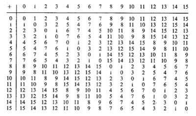Here’s the beginning of the nim-addition table on ordinals. For example, to define $13+7 $ we have to look at all values in the first 7 entries of the row of 13 (that is, ${ 13,12,15,14,9,8,11 } $) and the first 13 entries in the column of 7 (that is, ${ 7,6,5,4,3,2,1,0,15,14,13,12,11 } $) and find the first number not included in these two sets (which is indeed $10 $).

In fact, the above two rules allow us to compute the nim-sum of any two ordinals. Recall from last time that every ordinal can be written uniquely as as a finite sum of (ordinal) 2-powers :
$\alpha = [2^{\alpha_0} + 2^{\alpha_1} + \ldots + 2^{\alpha_k}] $, so to determine the nim-sum $\alpha+\beta $ we write both ordinals as sums of ordinal 2-powers, delete powers appearing twice and take the Cantor ordinal sum of the remaining sum.

Nim-multiplication of ordinals is a bit more complicated. Here’s the definition as a minimal excluded value

$\alpha.\beta = \mathbf{mex} { \alpha’.\beta + \alpha.\beta’ – \alpha’.\beta’ } $

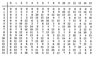
for all $\alpha’ < \alpha, \beta’ < \beta $. The rationale behind this being that both $\alpha-\alpha’ $ and $\beta – \beta’ $ are non-zero elements, so if $\mathbf{On}_2 $ is going to be a field under nim-multiplication, their product should be non-zero (and hence strictly greater than 0), that is, $~(\alpha-\alpha’).(\beta-\beta’) > 0 $. Rewriting this we get $\alpha.\beta > \alpha’.\beta+\alpha.\beta’-\alpha’.\beta’ $ and again the ‘simplicity rule’ asserts that $\alpha.\beta $ should be the least ordinal satisfying all these inequalities, leading to the $\mathbf{mex} $-definition above. The table gives the beginning of the nim-multiplication table for ordinals. For finite ordinals n and m there is a simple 2 line procedure to compute their nim-product, similar to the addition-rules mentioned before :

the nim-product of a number of distinct Fermat 2-powers (that is, numbers of the form $2^{2^n} $) is their ordinary product (for example, $16.4.2=128 $), and,
the square of a Fermat 2-power is its sesquimultiple (that is, the number obtained by multiplying with $1\frac{1}{2} $ in the ordinary sense). That is, $2^2=3,4^2=6,16^2=24,… $

Using these rules, associativity and distributivity and our addition rules it is now easy to work out the nim-multiplication $n.m $ : write out n and m as sums of (multiplications by 2-powers) of Fermat 2-powers and apply the rules. Here’s an example

$5.9=(4+1).(4.2+1)=4^2.2+4.2+4+1=6.2+8+4+1=(4+2).2+13=4.2+2^2+13=8+3+13=6 $

Clearly, we’d love to have a similar procedure to calculate the nim-product $\alpha.\beta $ of arbitrary ordinals, or at least those smaller than $\omega^{\omega^{\omega}} $ (recall that Conway proved that this ordinal is isomorphic to the algebraic closure $\overline{\mathbb{F}}_2 $ of the field of two elements). From now on we restrict to such ‘small’ ordinals and we introduce the following special elements :

$\kappa_{2^n} = [2^{2^{n-1}}] $ (these are the Fermat 2-powers) and for all primes $p > 2 $ we define
$\kappa_{p^n} = [\omega^{\omega^{k-1}.p^{n-1}}] $ where $k $ is the number of primes strictly smaller than $p $ (that is, for p=3 we have k=1, for p=5, k=2 etc.).

Again by associativity and distributivity we will be able to multiply two ordinals $< \omega^{\omega^{\omega}} $ if we know how to multiply a product

$[\omega^{\alpha}.2^{n_0}].[\omega^{\beta}.2^{m_0}] $ with $\alpha,\beta < [\omega^{\omega}] $ and $n_0,m_0 \in \mathbb{N} $.

Now, $\alpha $ can be written uniquely as $[\omega^t.n_t+\omega^{t-1}.n_{t-1}+\ldots+\omega.n_2 + n_1] $ with t and all $n_i $ natural numbers. Write each $n_k $ in base $p $ where $p $ is the $k+1 $-th prime number, that is, we have for $n_0,n_1,\ldots,n_t $ an expression

$n_k=[\sum_j p^j.m(j,k)] $ with $0 \leq m(j,k) < p $

The point of all this is that any of the special elements we want to multiply can be written as a unique expression as a decreasing product

$[\omega^{\alpha}.2^{n_0}] = [ \prod_q \kappa_q^m(q) ] $

where $q $ runs over all prime powers. The crucial fact now is that for this decreasing product we have a rule similar to addition of 2-powers, that is Conway-products coincide with the Cantor-products

$[ \prod_q \kappa_q^m(q) ] = \prod_q \kappa_q^m(q) $

But then, using associativity and commutativity of the Conway-product we can ‘nearly’ describe all products $[\omega^{\alpha}.2^{n_0}].[\omega^{\beta}.2^{m_0}] $. The remaining problem being that it may happen that for some q we will end up with an exponent $m(q)+m(q’)>p $. But this can be solved if we know how to take p-powers. The rules for this are as follows

$~(\kappa_{2^n})^2 = \kappa_{2^n} + \prod_{1 \leq i < n} \kappa_{2^i} $, for 2-powers, and,

$~(\kappa_{p^n})^p = \kappa_{p^{n-1}} $ for a prime $p > 2 $ and for $n \geq 2 $, and finally

$~(\kappa_p)^p = \alpha_p $ for a prime $p > 2 $, where $\alpha_p $ is the smallest ordinal $< \kappa_p $ which cannot be written as a p-power $\beta^p $ with $\beta < \kappa_p $. Summarizing : if we will be able to find these mysterious elements $\alpha_p $ for all prime numbers p, we are able to multiply in $[\omega^{\omega^{\omega}}]=\overline{\mathbb{F}}_2 $.

Let us determine the first one. We have that $\kappa_3 = \omega $ so we are looking for the smallest natural number $n < \omega $ which cannot be written in num-multiplication as $n=m^3 $ for $m < \omega $ (that is, also $m $ a natural number). Clearly $1=1^3 $ but what about 2? Can 2 be a third root of a natural number wrt. nim-multiplication? From the tabel above we see that 2 has order 3 whence its cube root must be an element of order 9. Now, the only finite ordinals that are subfields of $\mathbf{On}_2 $ are precisely the Fermat 2-powers, so if there is a finite cube root of 2, it must be contained in one of the finite fields $[2^{2^n}] $ (of which the mutiplicative group has order $2^{2^n}-1 $ and one easily shows that 9 cannot be a divisor of any of the numbers $2^{2^n}-1 $, that is, 2 doesn’t have a finte 3-th root in nim! Phrased differently, we found our first mystery number $\alpha_3 = 2 $. That is, we have the marvelous identity in nim-arithmetic

$\omega^3 = 2 $

Okay, so what is $\alpha_5 $? Well, we have $\kappa_5 = [\omega^{\omega}] $ and we have to look for the smallest ordinal which cannot be written as a 5-th root. By inspection of the finite nim-table we see that 1,2 and 3 have 5-th roots in $\omega $ but 4 does not! The reason being that 4 has order 15 (check in the finite field [16]) and 25 cannot divide any number of the form $2^{2^n}-1 $. That is, $\alpha_5=4 $ giving another crazy nim-identity

$~(\omega^{\omega})^5 = 4 $

And, surprises continue to pop up… Conway showed that $\alpha_7 = \omega+1 $ giving the nim-identity $~(\omega^{\omega^2})^7 = \omega+1 $. The proof of this already uses some clever finite field arguments. Because 7 doesn’t divide any number $2^{2^n}-1 $, none of the finite subfields $[2^{2^n}] $ contains a 7-th root of unity, so the 7-power map is injective whence surjective, so all finite ordinal have finite 7-th roots! That is, $\alpha_7 \geq \omega $. Because $\omega $ lies in a cubic extension of the finite field [4], the field generated by $\omega $ has 64 elements and so its multiplicative group is cyclic of order 63 and as $\omega $ has order 9, it must be a 7-th power in this field. But, as the only 7th powers in that field are precisely the powers of $\omega $ and by inspection $\omega+1 $ is not a 7-th power in that field (and hence also not in any field extension obtained by adjoining square, cube and fifth roots) so $\alpha_7=\omega +1 $.

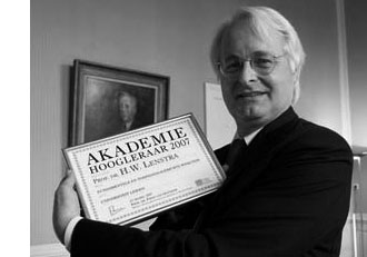
Conway did stop at $\alpha_7 $ but I’ve always been intrigued by that one line in ONAG p.61 : “Hendrik Lenstra has computed $\alpha_p $ for $p \leq 43 $”. Next time we will see how Lenstra managed to do this and we will use sage to extend his list a bit further, including the first open case : $\alpha_{47}= \omega^{\omega^7}+1 $.

For an enjoyable video on all of this, see Conway’s MSRI lecture on Infinite Games. The nim-arithmetic part is towards the end of the lecture but watching the whole video is a genuine treat!