These three ideas (re)surfaced over the last two decades, claiming to have potential applications to major open problems:
- (2000) $\mathbb{F}_1$-geometry tries to view $\mathbf{Spec}(\mathbb{Z})$ as a curve over the field with one element, and mimic Weil’s proof of RH for curves over finite fields to prove the Riemann hypothesis.
- (2012) IUTT, for Inter Universal Teichmuller Theory, the machinery behind Mochizuki’s claimed proof of the ABC-conjecture.
- (2014) topos theory : Connes and Consani redirected their RH-attack using arithmetic sites, while Lafforgue advocated the use of Caramello’s bridges for unification, in particular the Langlands programme.
It is difficult to voice an opinion about the (presumed) current state of such projects without being accused of being either a believer or a skeptic, resorting to group-think or being overly critical.
We lack the vocabulary to talk about the different phases a mathematical idea might be in.
Such a vocabulary exists in (information) technology, the five phases of the Gartner hype cycle to represent the maturity, adoption, and social application of a certain technology :
- Technology Trigger
- Peak of Inflated Expectations
- Trough of Disillusionment
- Slope of Enlightenment
- Plateau of Productivity
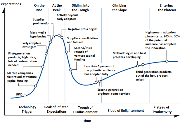
This model can then be used to gauge in which phase several emerging technologies are, and to estimate the time it will take them to reach the stable plateau of productivity. Here’s Gartner’s recent Hype Cycle for emerging Artificial Intelligence technologies.
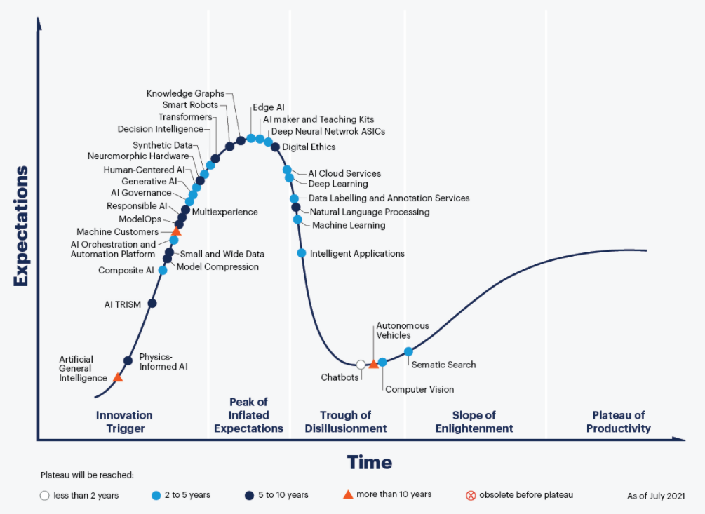
Picture from Gartner Hype Cycle for AI 2021
What might these phases be in the hype cycle of a mathematical idea?
- Technology Trigger: a new idea or analogy is dreamed up, marketed to be the new approach to that problem. A small group of enthusiasts embraces the idea, and tries to supply proper definitions and the very first results.
- Peak of Inflated Expectations: the idea spreads via talks, blogposts, mathoverflow and twitter, and now has enough visibility to justify the first conferences devoted to it. However, all this activity does not result in major breakthroughs and doubt creeps in.
- Trough of Disillusionment: the project ran out of steam. It becomes clear that existing theories will not lead to a solution of the motivating problem. Attempts by key people to keep the idea alive (by lengthy papers, regular meetings or seminars) no longer attract new people to the field.
- Slope of Enlightenment: the optimistic scenario. One abandons the original aim, ditches the myriad of theories leading nowhere, regroups and focusses on the better ideas the project delivered.
A negative scenario is equally possible. Apart for a few die-hards the idea is abandoned, and on its way to the graveyard of forgotten ideas.
- Plateau of Productivity: the polished surviving theory has applications in other branches and becomes a solid tool in mathematics.
It would be fun so see more knowledgable people draw such a hype cycle graph for recent trends in mathematics.
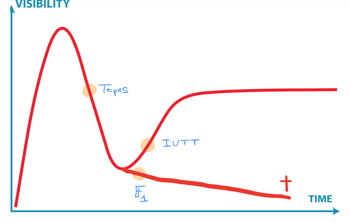
Here’s my own (feeble) attempt to gauge where the three ideas mentioned at the start are in their cycles, and here’s why:
- IUTT: recent work of Kirti Joshi, for example this, and this, and that, draws from IUTT while using conventional language and not making exaggerated claims.
- $\mathbb{F}_1$: the preliminary programme of their seminar shows little evidence the $\mathbb{F}_1$-community learned from the past 20 years.
- Topos: Developing more general theory is not the way ahead, but concrete examples may carry surprises, even though Gabriel’s topos will remain elusive.
Clearly, you don’t agree, and that’s fine. We now have a common terminology, and you can point me to results or events I must have missed, forcing me to redraw my graph.
Leave a Comment