Author: lievenlb

Mumford’s treasure map

Published December 13, 2008 by lievenlb

David Mumford did receive earlier this year the 2007 AMS Leroy P. Steele Prize for Mathematical Exposition. The jury honors Mumford for “his beautiful expository accounts of a host of aspects of algebraic geometry”. Not surprisingly, the first work they mention are his mimeographed notes of the first 3 chapters of a course in algebraic geometry, usually called “Mumford’s red book” because the notes were wrapped in a red cover. In 1988, the notes were reprinted by Springer-Verlag. Unfortnately, the only red they preserved was in the title.

The AMS describes the importance of the red book as follows. “This is one of the few books that attempt to convey in pictures some of the highly abstract notions that arise in the field of algebraic geometry. In his response upon receiving the prize, Mumford recalled that some of his drawings from The Red Book were included in a collection called Five Centuries of French Mathematics. This seemed fitting, he noted: “After all, it was the French who started impressionist painting and isn’t this just an impressionist scheme for rendering geometry?””

These days it is perfectly possible to get a good grasp on difficult concepts from algebraic geometry by reading blogs, watching YouTube or plugging in equations to sophisticated math-programs. In the early seventies though, if you wanted to know what Grothendieck’s scheme-revolution was all about you had no choice but to wade through the EGA’s and SGA’s and they were notorious for being extremely user-unfriendly regarding illustrations…

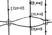
So the few depictions of schemes available, drawn by people sufficiently fluent in Grothendieck’s new geometric language had no less than treasure-map-cult-status and were studied in minute detail. Mumford’s red book was a gold mine for such treasure maps. Here’s my favorite one, scanned from the original mimeographed notes (it looks somewhat tidier in the Springer-version)

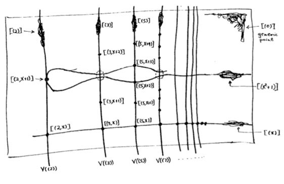
It is the first depiction of $\mathbf{spec}(\mathbb{Z}[x]) $, the affine scheme of the ring $\mathbb{Z}[x] $ of all integral polynomials. Mumford calls it the”arithmetic surface” as the picture resembles the one he made before of the affine scheme $\mathbf{spec}(\mathbb{C}[x,y]) $ corresponding to the two-dimensional complex affine space $\mathbb{A}^2_{\mathbb{C}} $. Mumford adds that the arithmetic surface is ‘the first example which has a real mixing of arithmetic and geometric properties’.

Let’s have a closer look at the treasure map. It introduces some new signs which must have looked exotic at the time, but have since become standard tools to depict algebraic schemes.

For starters, recall that the underlying topological space of $\mathbf{spec}(\mathbb{Z}[x]) $ is the set of all prime ideals of the integral polynomial ring $\mathbb{Z}[x] $, so the map tries to list them all as well as their inclusions/intersections.

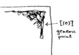The doodle in the right upper corner depicts the ‘generic point’ of the scheme. That is, the geometric object corresponding to the prime ideal $~(0) $ (note that $\mathbb{Z}[x] $ is an integral domain). Because the zero ideal is contained in any other prime ideal, the algebraic/geometric mantra (“inclusions reverse when shifting between algebra and geometry”) asserts that the gemetric object corresponding to $~(0) $ should contain all other geometric objects of the arithmetic plane, so it is just the whole plane! Clearly, it is rather senseless to depict this fact by coloring the whole plane black as then we wouldn’t be able to see the finer objects. Mumford’s solution to this is to draw a hairy ball, which in this case, is sufficiently thick to include fragments going in every possible direction. In general, one should read these doodles as saying that the geometric object represented by this doodle contains all other objects seen elsewhere in the picture if the hairy-ball-doodle includes stuff pointing in the direction of the smaller object. So, in the case of the object corresponding to $~(0) $, the doodle has pointers going everywhere, saying that the geometric object contains all other objects depicted.

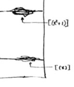Let’s move over to the doodles in the lower right-hand corner. They represent the geometric object corresponding to principal prime ideals of the form $~(p(x)) $, where $p(x) $ in an irreducible polynomial over the integers, that is, a polynomial which we cannot write as the product of two smaller integral polynomials. The objects corresponding to such prime ideals should be thought of as ‘horizontal’ curves in the plane.

The doodles depicted correspond to the prime ideal $~(x) $, containing all polynomials divisible by $x $ so when we divide it out we get, as expected, a domain $\mathbb{Z}[x]/(x) \simeq \mathbb{Z} $, and the one corresponding to the ideal $~(x^2+1) $, containing all polynomials divisible by $x^2+1 $, which can be proved to be a prime ideals of $\mathbb{Z}[x] $ by observing that after factoring out we get $\mathbb{Z}[x]/(x^2+1) \simeq \mathbb{Z}[i] $, the domain of all Gaussian integers $\mathbb{Z}[i] $. The corresponding doodles (the ‘generic points’ of the curvy-objects) have a predominant horizontal component as they have the express the fact that they depict horizontal curves in the plane. It is no coincidence that the doodle of $~(x^2+1) $ is somewhat bulkier than the one of $~(x) $ as the later one must only depict the fact that all points lying on the straight line to its left belong to it, whereas the former one must claim inclusion of all points lying on the ‘quadric’ it determines.

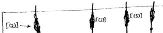Apart from these ‘horizontal’ curves, there are also ‘vertical’ lines corresponding to the principal prime ideals $~(p) $, containing the polynomials, all of which coefficients are divisible by the prime number $p $. These are indeed prime ideals of $\mathbb{Z}[x] $, because their quotients are
$\mathbb{Z}[x]/(p) \simeq (\mathbb{Z}/p\mathbb{Z})[x] $ are domains, being the ring of polynomials over the finite field $\mathbb{Z}/p\mathbb{Z} = \mathbb{F}_p $. The doodles corresponding to these prime ideals have a predominant vertical component (depicting the ‘vertical’ lines) and have a uniform thickness for all prime numbers $p $ as each of them only has to claim ownership of the points lying on the vertical line under them.

Right! So far we managed to depict the zero prime ideal (the whole plane) and the principal prime ideals of $\mathbb{Z}[x] $ (the horizontal curves and the vertical lines). Remains to depict the maximal ideals. These are all known to be of the form
$\mathfrak{m} = (p,f(x)) $
where $p $ is a prime number and $f(x) $ is an irreducible integral polynomial, which remains irreducible when reduced modulo $p $ (that is, if we reduce all coefficients of the integral polynomial $f(x) $ modulo $p $ we obtain an irreducible polynomial in $~\mathbb{F}_p[x] $). By the algebra/geometry mantra mentioned before, the geometric object corresponding to such a maximal ideal can be seen as the ‘intersection’ of an horizontal curve (the object corresponding to the principal prime ideal $~(f(x)) $) and a vertical line (corresponding to the prime ideal $~(p) $). Because maximal ideals do not contain any other prime ideals, there is no reason to have a doodle associated to $\mathfrak{m} $ and we can just depict it by a “point” in the plane, more precisely the intersection-point of the horizontal curve with the vertical line determined by $\mathfrak{m}=(p,f(x)) $. Still, Mumford’s treasure map doesn’t treat all “points” equally. For example, the point corresponding to the maximal ideal $\mathfrak{m}_1 = (3,x+2) $ is depicted by a solid dot $\mathbf{.} $, whereas the point corresponding to the maximal ideal $\mathfrak{m}_2 = (3,x^2+1) $ is represented by a fatter point $\circ $. The distinction between the two ‘points’ becomes evident when we look at the corresponding quotients (which we know have to be fields). We have

$\mathbb{Z}[x]/\mathfrak{m}_1 = \mathbb{Z}[x]/(3,x+2)=(\mathbb{Z}/3\mathbb{Z})[x]/(x+2) = \mathbb{Z}/3\mathbb{Z} = \mathbb{F}_3 $ whereas $\mathbb{Z}[x]/\mathfrak{m}_2 = \mathbb{Z}[x]/(3,x^2+1) = \mathbb{Z}/3\mathbb{Z}[x]/(x^2+1) = \mathbb{F}_3[x]/(x^2+1) = \mathbb{F}_{3^2} $

because the polynomial $x^2+1 $ remains irreducible over $\mathbb{F}_3 $, the quotient $\mathbb{F}_3[x]/(x^2+1) $ is no longer the prime-field $\mathbb{F}_3 $ but a quadratic field extension of it, that is, the finite field consisting of 9 elements $\mathbb{F}_{3^2} $. That is, we represent the ‘points’ lying on the vertical line corresponding to the principal prime ideal $~(p) $ by a solid dot . when their quotient (aka residue field is the prime field $~\mathbb{F}_p $, by a bigger point $\circ $ when its residue field is the finite field $~\mathbb{F}_{p^2} $, by an even fatter point $\bigcirc $ when its residue field is $~\mathbb{F}_{p^3} $ and so on, and on. The larger the residue field, the ‘fatter’ the corresponding point.

In fact, the ‘fat-point’ signs in Mumford’s treasure map are an attempt to depict the fact that an affine scheme contains a lot more information than just the set of all prime ideals. In fact, an affine scheme determines (and is determined by) a “functor of points”. That is, to every field (or even every commutative ring) the affine scheme assigns the set of its ‘points’ defined over that field (or ring). For example, the $~\mathbb{F}_p $-points of $\mathbf{spec}(\mathbb{Z}[x]) $ are the solid . points on the vertical line $~(p) $, the $~\mathbb{F}_{p^2} $-points of $\mathbf{spec}(\mathbb{Z}[x]) $ are the solid . points and the slightly bigger $\circ $ points on that vertical line, and so on.

This concludes our first attempt to decypher Mumford’s drawing, but if we delve a bit deeper, we are bound to find even more treasures… (to be continued).

5 Comments

beyond the blog

Published December 7, 2008 by lievenlb

For starters, apologies for flooding your RSS-aggregators a couple of days ago. Ive been copying my posts at F_un mathematics and have cross-posted them here. I will continue to do so as I prefer to search just one blog instead of two to find stuff. Besides, it’s unclear how long the F_un site will survive. Javier will be moving from MPI to London later this month, and is uncertain on the implications this will have for his research. Other people who told they’d like to post at F_un haven’t done so far… and I see little point in continuing a singleton-‘group blog’.

Over at the secret blogging seminar there is an interesting series on TQFTs via planar algebras by Chris Schommer-Pries. They also had a few nice words on the design of the F_un-site (though their commenters prefer a ‘traditional’ blog-layout). I think these days most people read blogs via their RSS-feeds, so are ignorant about the actual layout of a blog until they want to follow up a story that interests them. Besides, the main point of using the open book wordpress theme, which is a so called ‘magazine’-theme, was to try to get more structure in the blog (such as : indicating the intented audience for a post, organizing posts wrt. the papers mentioned etc.). Still, such themes are designed for news-sites having new content every hour/day, something we cannot say of the F_un-site…

Also at the n-category cafe they are thinking aloud on how to improve the blog-medium for mathematics-research. See the discussion following David Corfield’s beyond the blog post. Often, the comment-thread of an n-cafe post is a better read than the actual post, but the blog-concept is not very good at picking-out interesting comments. That’s why they are trying to set up a wiki-like thing with pointers to such interesting discussions. It’s still early days but they’ve started the nLab (powered by instiki) and describe it as “this place is like the library, or alchemist’s laboratory, in the back room of the n-Category Café. You come here to work and go there to chat”. Surely an interesting experiment to follow.

Finally, a link to images des mathematiques which is a news-site-style blog on mathematics run by the CNRS (the French NSF). They give their posts ‘colours’, indicating the intented public, surely a simple idea we can all implement that will make math-blogs a lot more useful. They also have repeating topics, such as ‘the object of the month’, portraits of mathematicians etc. Perhaps an idea to follow-up by other math-societies.

If you have ideas to improve the structure and usability of math-blogs, please share them!

noncommutative F_un geometry (2)

Published October 17, 2008 by lievenlb

Last time we tried to generalize the Connes-Consani approach to commutative algebraic geometry over the field with one element $\mathbb{F}_1 $ to the noncommutative world by considering covariant functors

$N~:~\mathbf{groups} \rightarrow \mathbf{sets} $

which over $\mathbb{C} $ resp. $\mathbb{Z} $ become visible by a complex (resp. integral) algebra having suitable universal properties.

However, we didn’t specify what we meant by a complex noncommutative variety (resp. an integral noncommutative scheme). In particular, we claimed that the $\mathbb{F}_1 $-‘points’ associated to the functor

$D~:~\mathbf{groups} \rightarrow \mathbf{sets} \qquad G \mapsto G_2 \times G_3 $ (here $G_n $ denotes all elements of order $n $ of $G $)

were precisely the modular dessins d’enfants of Grothendieck, but didn’t give details. We’ll try to do this now.

For algebras over a field we follow the definition, due to Kontsevich and Soibelman, of so called “noncommutative thin schemes”. Actually, the thinness-condition is implicit in both Soule’s-approach as that of Connes and Consani : we do not consider R-points in general, but only those of rings R which are finite and flat over our basering (or field).

So, what is a noncommutative thin scheme anyway? Well, its a covariant functor (commuting with finite projective limits)

$\mathbb{X}~:~\mathbf{Alg}^{fd}_k \rightarrow \mathbf{sets} $

from finite-dimensional (possibly noncommutative) $k $-algebras to sets. Now, the usual dual-space operator gives an anti-equivalence of categories

$\mathbf{Alg}^{fd}_k \leftrightarrow \mathbf{Coalg}^{fd}_k \qquad A=C^* \leftrightarrow C=A^* $

so a thin scheme can also be viewed as a contra-variant functor (commuting with finite direct limits)

$\mathbb{X}~:~\mathbf{Coalg}^{fd}_k \rightarrow \mathbf{Sets} $

In particular, we are interested to associated to any {tex]k $-algebra $A $ its representation functor :

$\mathbf{rep}(A)~:~\mathbf{Coalg}^{fd}_k \rightarrow \mathbf{Sets} \qquad C \mapsto Alg_k(A,C^*) $

This may look strange at first sight, but $C^* $ is a finite dimensional algebra and any $n $-dimensional representation of $A $ is an algebra map $A \rightarrow M_n(k) $ and we take $C $ to be the dual coalgebra of this image.

Kontsevich and Soibelman proved that every noncommutative thin scheme $\mathbb{X} $ is representable by a $k $-coalgebra. That is, there exists a unique coalgebra $C_{\mathbb{X}} $ (which they call the coalgebra of ‘distributions’ of $\mathbb{X} $) such that for every finite dimensional $k $-algebra $B $ we have

$\mathbb{X}(B) = Coalg_k(B^*,C_{\mathbb{X}}) $

In the case of interest to us, that is for the functor $\mathbf{rep}(A) $ the coalgebra of distributions is Kostant’s dual coalgebra $A^o $. This is the not the full linear dual of $A $ but contains only those linear functionals on $A $ which factor through a finite dimensional quotient.

So? You’ve exchanged an algebra $A $ for some coalgebra $A^o $, but where’s the geometry in all this? Well, let’s look at the commutative case. Suppose $A= \mathbb{C}[X] $ is the coordinate ring of a smooth affine variety $X $, then its dual coalgebra looks like

$\mathbb{C}[X]^o = \oplus_{x \in X} U(T_x(X)) $

the direct sum of all universal (co)algebras of tangent spaces at points $x \in X $. But how do we get the variety out of this? Well, any coalgebra has a coradical (being the sun of all simple subcoalgebras) and in the case just mentioned we have

$corad(\mathbb{C}[X]^o) = \oplus_{x \in X} \mathbb{C} e_x $

so every point corresponds to a unique simple component of the coradical. In the general case, the coradical of the dual coalgebra $A^o $ is the direct sum of all simple finite dimensional representations of $A $. That is, the direct summands of the coalgebra give us a noncommutative variety whose points are the simple representations, and the remainder of the coalgebra of distributions accounts for infinitesimal information on these points (as do the tangent spaces in the commutative case).

In fact, it was a surprise to me that one can describe the dual coalgebra quite explicitly, and that $A_{\infty} $-structures make their appearance quite naturally. See this paper if you’re in for the details on this.

That settles the problem of what we mean by the noncommutative variety associated to a complex algebra. But what about the integral case? In the above, we used extensively the theory of Kostant-duality which works only for algebras over fields…

Well, not quite. In the case of $\mathbb{Z} $ (or more general, of Dedekind domains) one can repeat Kostant’s proof word for word provided one takes as the definition of the dual $\mathbb{Z} $-coalgebra
of an algebra (which is $\mathbb{Z} $-torsion free)

$A^o = { f~:~A \rightarrow \mathbb{Z}~:~A/Ker(f)~\text{is finitely generated and torsion free}~} $

(over general rings there may be also variants of this duality, as in Street’s book an Quantum groups). Probably lots of people have come up with this, but the only explicit reference I have is to the first paper I’ve ever written. So, also for algebras over $\mathbb{Z} $ we can define a suitable noncommutative integral scheme (the coradical approach accounts only for the maximal ideals rather than all primes, but somehow this is implicit in all approaches as we consider only thin schemes).

Fine! So, we can make sense of the noncommutative geometrical objects corresponding to the group-algebras $\mathbb{C} \Gamma $ and $\mathbb{Z} \Gamma $ where $\Gamma = PSL_2(\mathbb{Z}) $ is the modular group (the algebras corresponding to the $G \mapsto G_2 \times G_3 $-functor). But, what might be the points of the noncommutative scheme corresponding to $\mathbb{F}_1 \Gamma $???

Well, let’s continue the path cut out before. “Points” should correspond to finite dimensional “simple representations”. Hence, what are the finite dimensional simple $\mathbb{F}_1 $-representations of $\Gamma $? (Or, for that matter, of any group $G $)

Here we come back to Javier’s post on this : a finite dimensional $\mathbb{F}_1 $-vectorspace is a finite set. A $\Gamma $-representation on this set (of n-elements) is a group-morphism

$\Gamma \rightarrow GL_n(\mathbb{F}_1) = S_n $

hence it gives a permutation representation of $\Gamma $ on this set. But then, if finite dimensional $\mathbb{F}_1 $-representations of $\Gamma $ are the finite permutation representations, then the simple ones are the transitive permutation representations. That is, the points of the noncommutative scheme corresponding to $\mathbb{F}_1 \Gamma $ are the conjugacy classes of subgroups $H \subset \Gamma $ such that $\Gamma/H $ is finite. But these are exactly the modular dessins d’enfants introduced by Grothendieck as I explained a while back elsewhere (see for example this post and others in the same series).